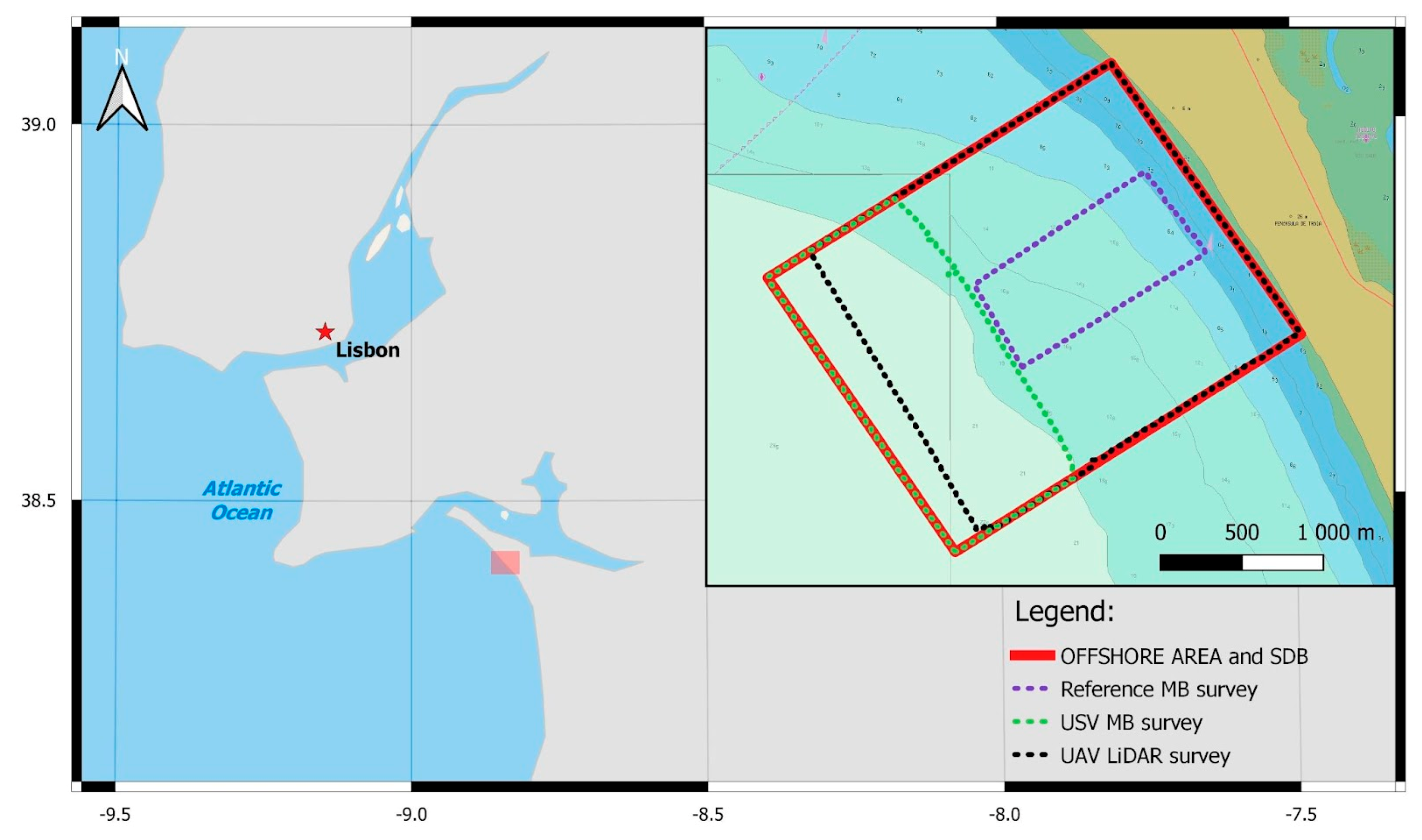
figure 1.
Overview of the survey area.
figure 1.
Overview of the survey area.
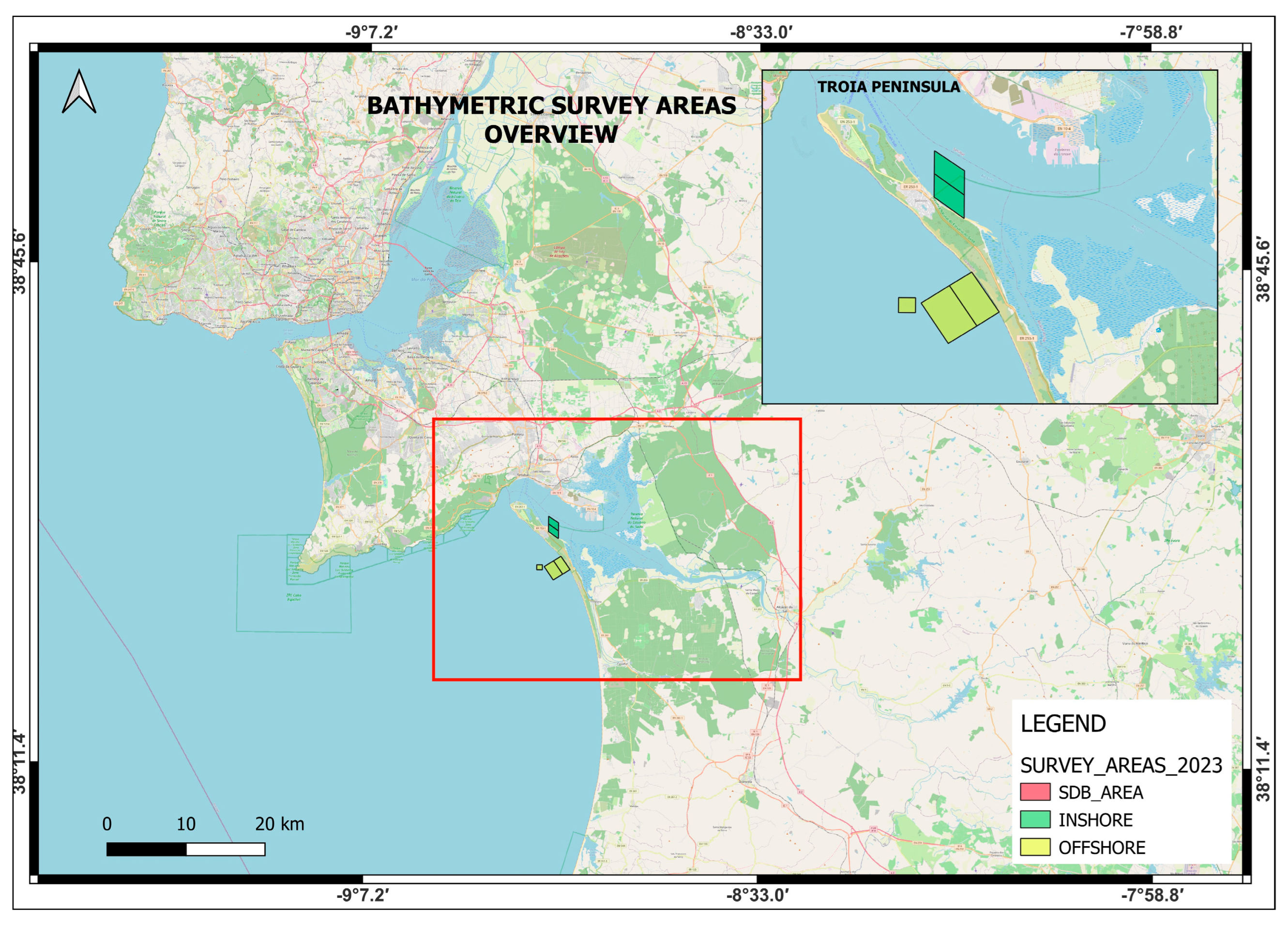
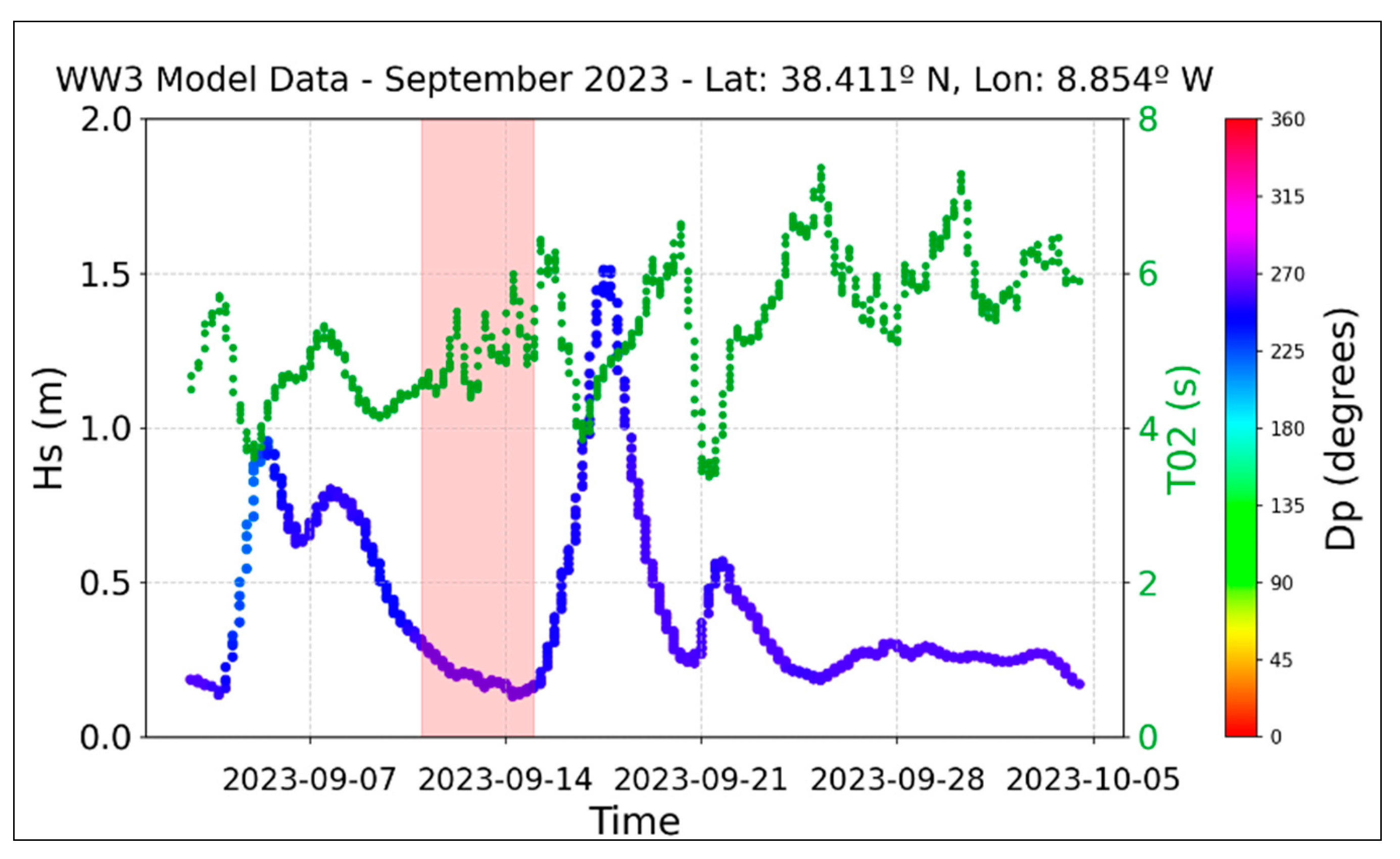
figure 2.
Meteorological conditions in the study area – significant wave height (Hs), wave period (T02) and wave direction (Dp) in the WW3 model during the survey period (red area).
figure 2.
Meteorological conditions in the study area – significant wave height (Hs), wave period (T02) and wave direction (Dp) in the WW3 model during the survey period (red area).
Siebel CAMCOPTER® S-100 equipped with Areté PILLS (RAMMS) lidar system [41].
Siebel CAMCOPTER® S-100 equipped with Areté PILLS (RAMMS) lidar system [41].
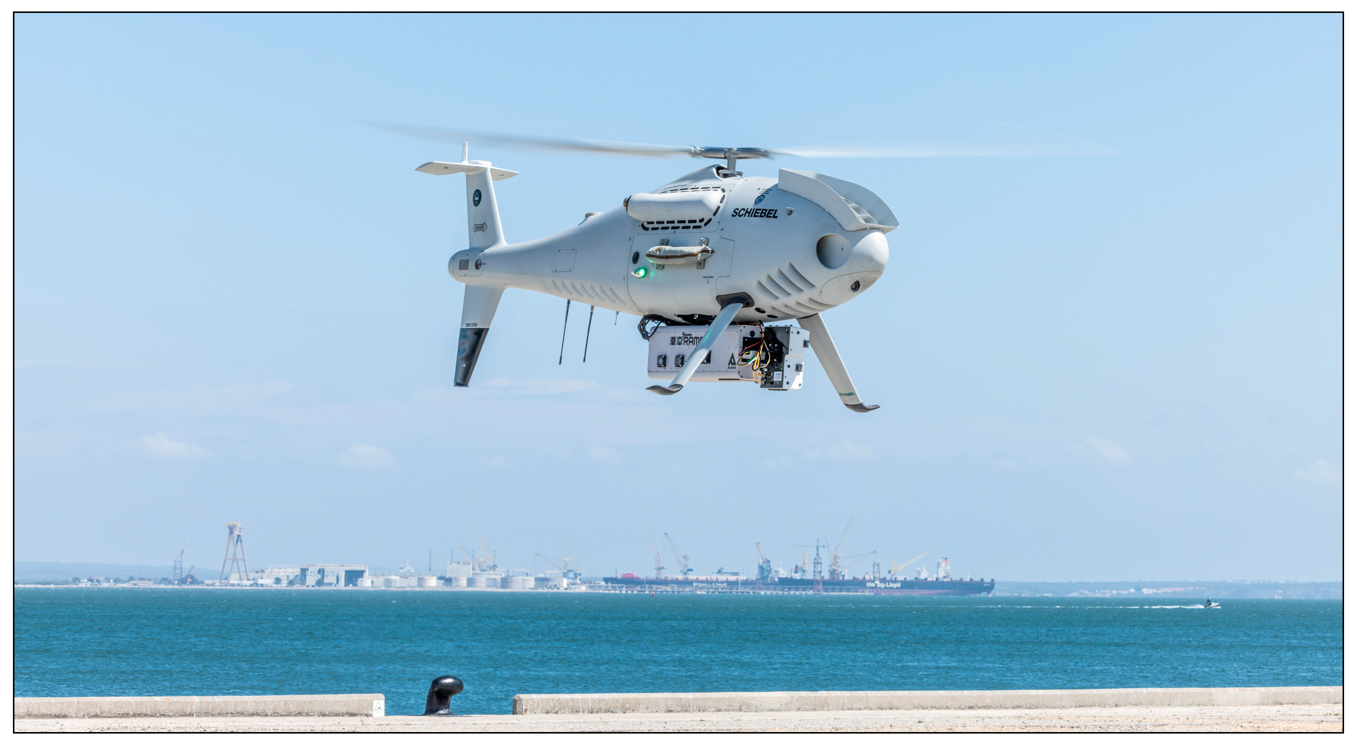
Figure 4.
Hydrographic measurements by the DriX USV during the REPMUS23 exercise.
Figure 4.
Hydrographic measurements by the DriX USV during the REPMUS23 exercise.
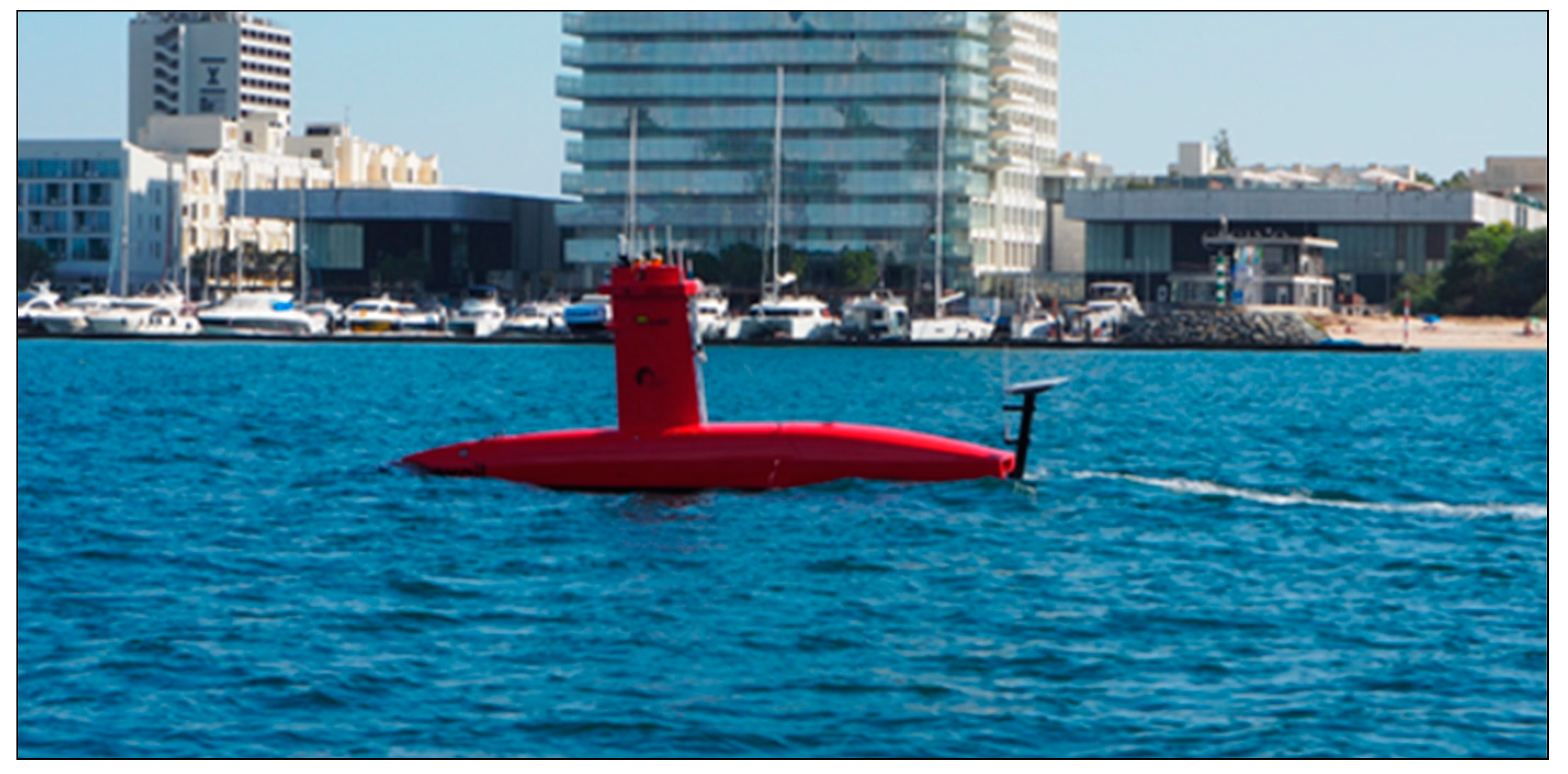
Figure 5.
DriX USV’s patch test survey line.
Figure 5.
DriX USV’s patch test survey line.
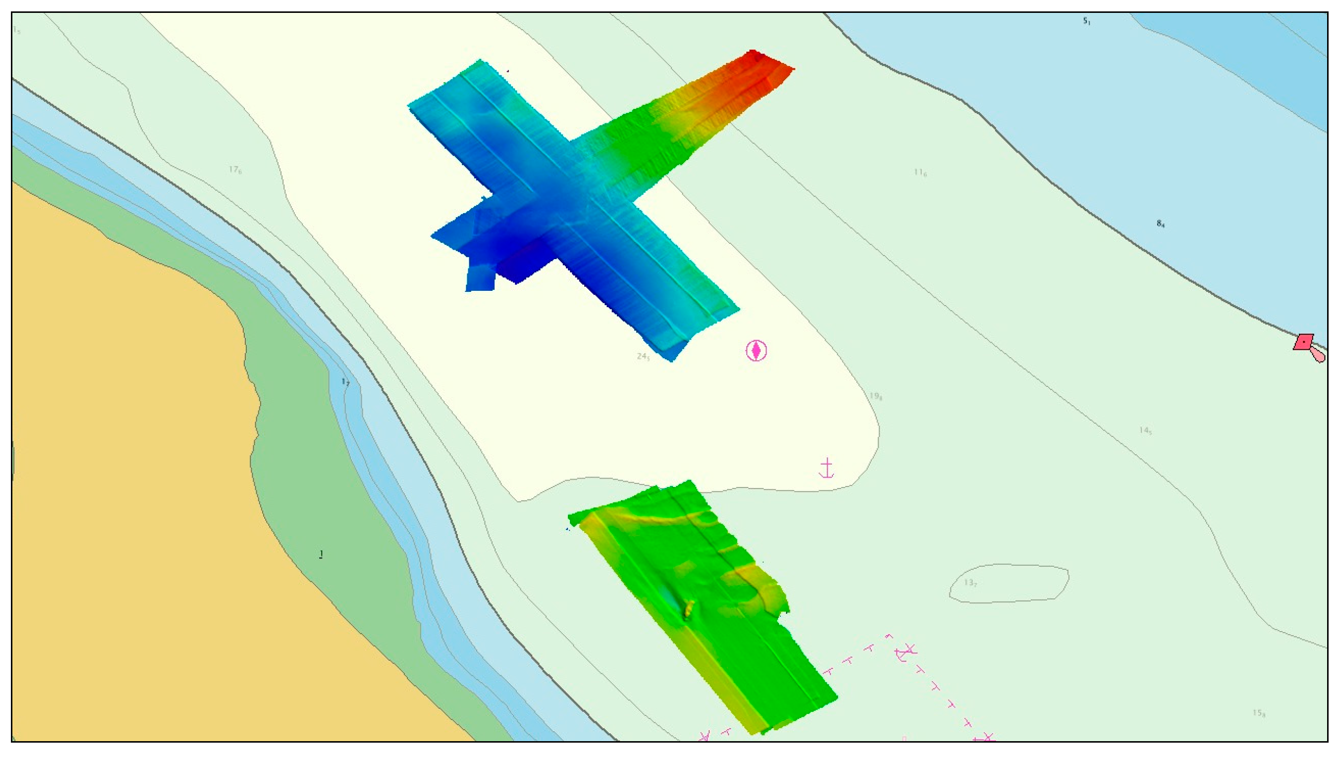
Figure 6.
A subset of the DriX USV multibeam data shows that sound speeds have been sampled and applied correctly, resulting in a correct representation of the flat seafloor (each color represents a different survey line).
Figure 6.
A subset of the DriX USV multibeam data shows that sound speeds have been sampled and applied correctly, resulting in a correct representation of the flat seafloor (each color represents a different survey line).
Figure 7.
A subset of the reference survey multibeam data shows that sound speeds have been correctly sampled and applied, resulting in a correct representation of the flat seafloor (each color represents a different survey line).
Figure 7.
A subset of the reference survey multibeam data shows that sound speeds have been correctly sampled and applied, resulting in a correct representation of the flat seafloor (each color represents a different survey line).
Figure 8.
Overview plots depict the general location of the offshore areas, as well as a detailed plan representing the bathymetric coverage for each data set.
Figure 8.
Overview plots depict the general location of the offshore areas, as well as a detailed plan representing the bathymetric coverage for each data set.
Tide tables used to show tide heights during measurements.Can be used as [57].
Tide tables used to show tide heights during measurements.Can be used as [57].
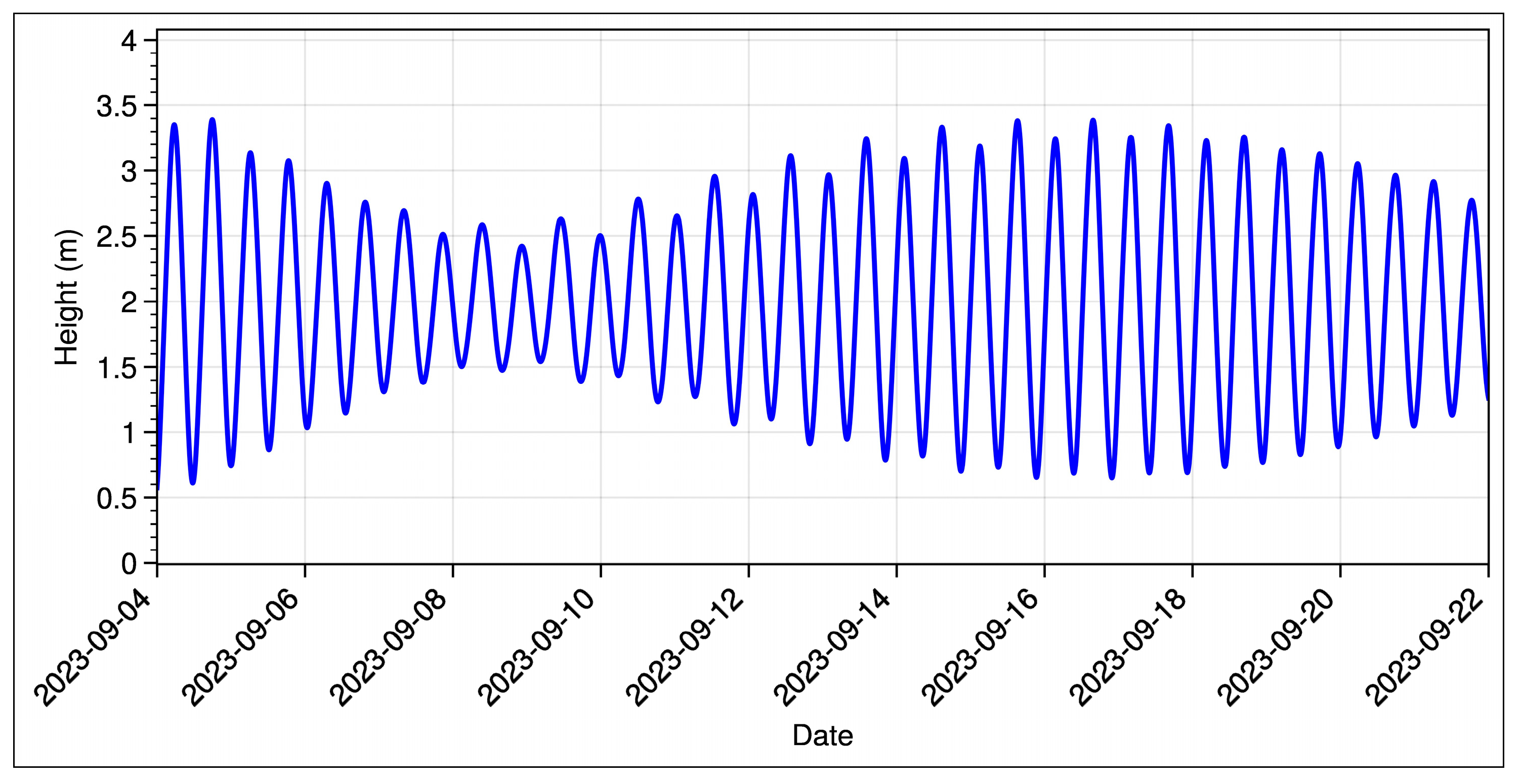
Figure 10.
Reference bathymetric surface.
Figure 10.
Reference bathymetric surface.
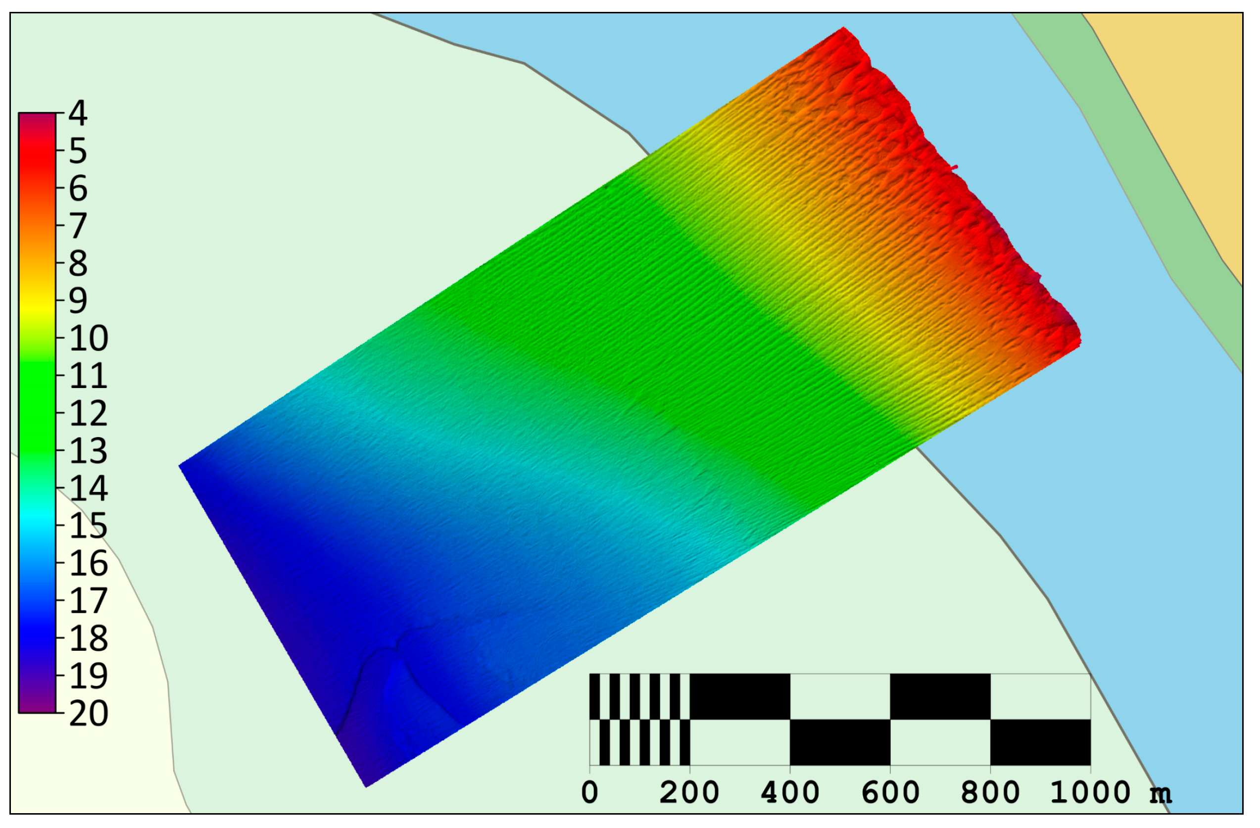
Figure 11.
Reference bathymetry statistics, (A)——Node density, (Second)——node standard deviation.
Figure 11.
Reference bathymetry statistics, (A)——Node density, (Second)——node standard deviation.
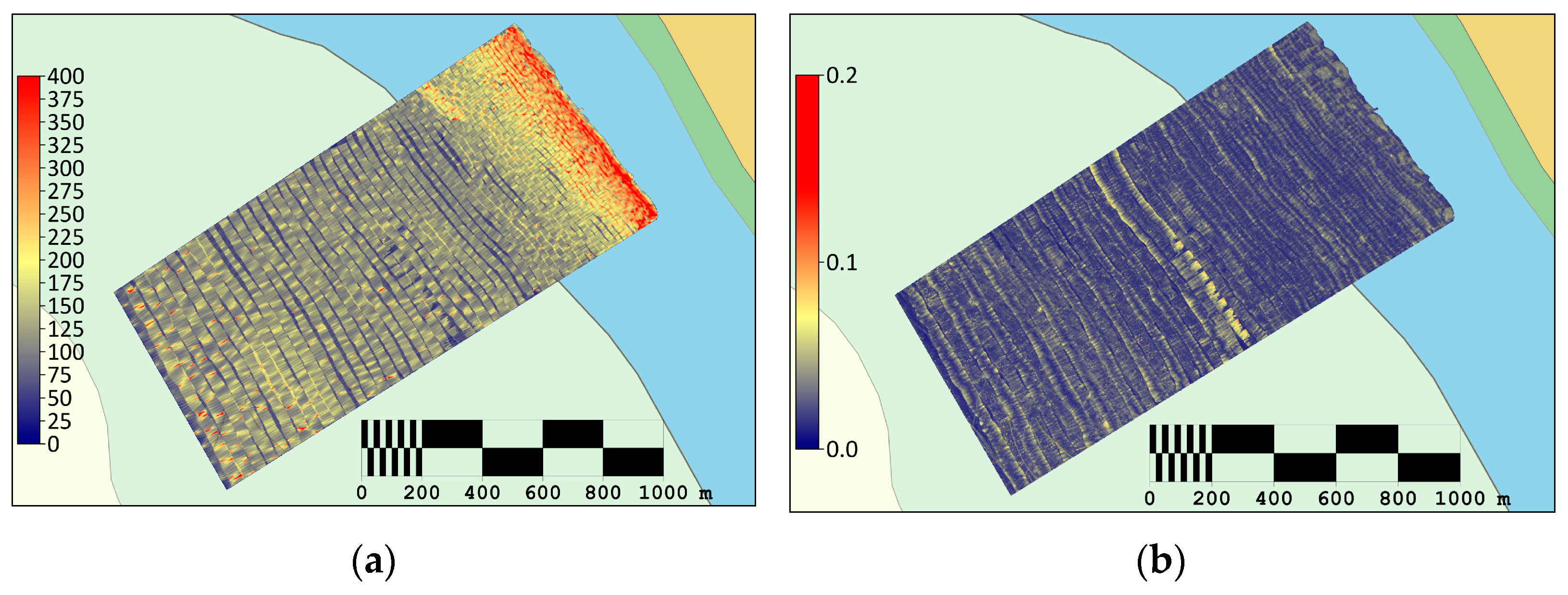
Figure 12.
USV MB bathymetric surface.
Figure 12.
USV MB bathymetric surface.
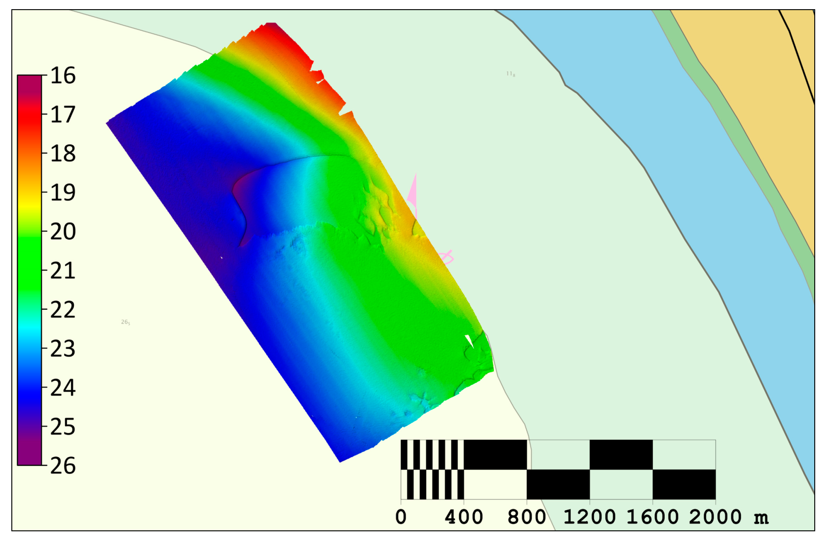
Figure 13.
USV MB bathymetry statistics, (A)——Node density, (Second)——node standard deviation.
Figure 13.
USV MB bathymetry statistics, (A)——Node density, (Second)——node standard deviation.
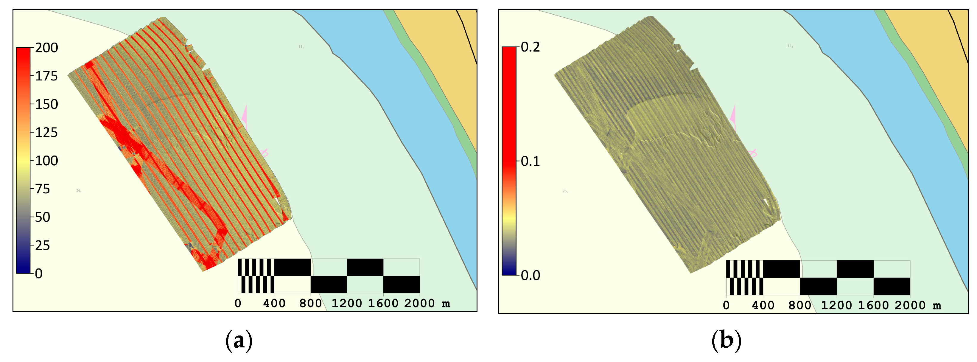
Figure 14.
Drone lidar bathymetric surface.
Figure 14.
Drone lidar bathymetric surface.
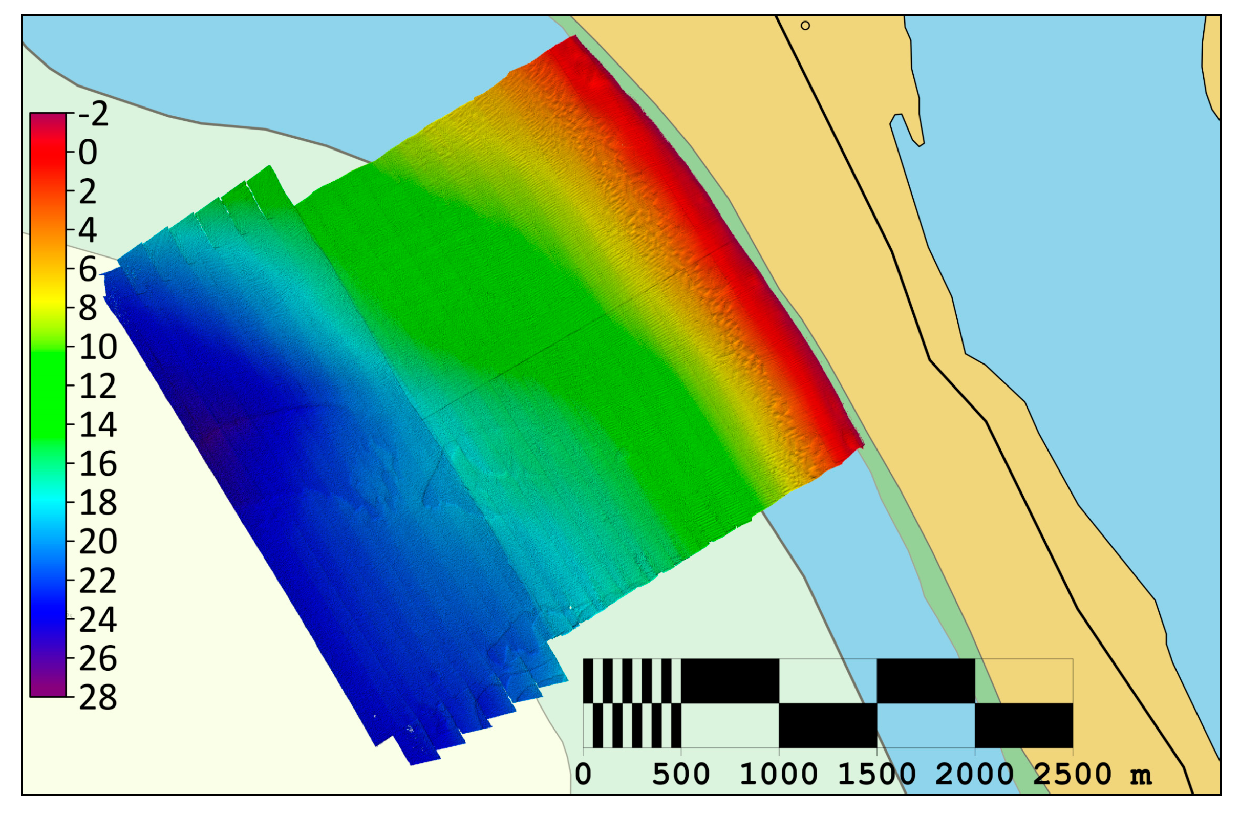
Figure 15.
UAV lidar bathymetric survey statistics, (A)——Node density, (Second)——node standard deviation.
Figure 15.
UAV lidar bathymetric survey statistics, (A)——Node density, (Second)——node standard deviation.
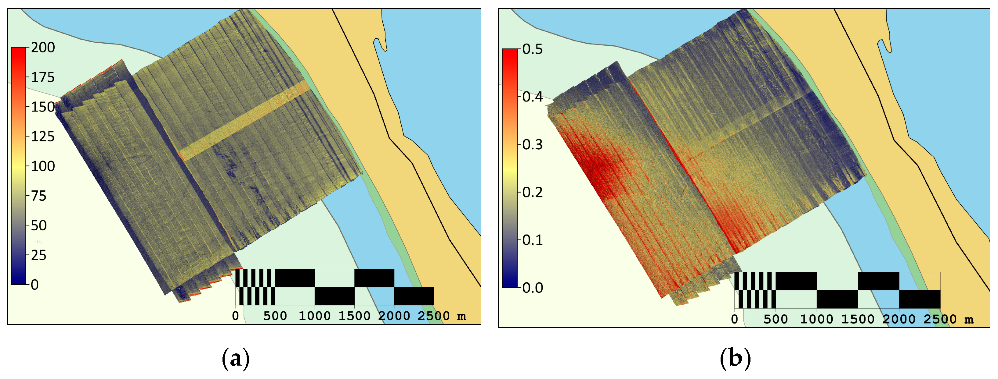
Figure 16.
(A)—the position of the vertical transverse profile between the shallow surface and the deep surface (Second)—Inconsistent step between shallow and deep LiDAR UAV surfaces (for contours selected between two colored squares).
Figure 16.
(A)—the position of the vertical transverse profile between the shallow surface and the deep surface (Second)—Inconsistent step between shallow and deep LiDAR UAV surfaces (for contours selected between two colored squares).
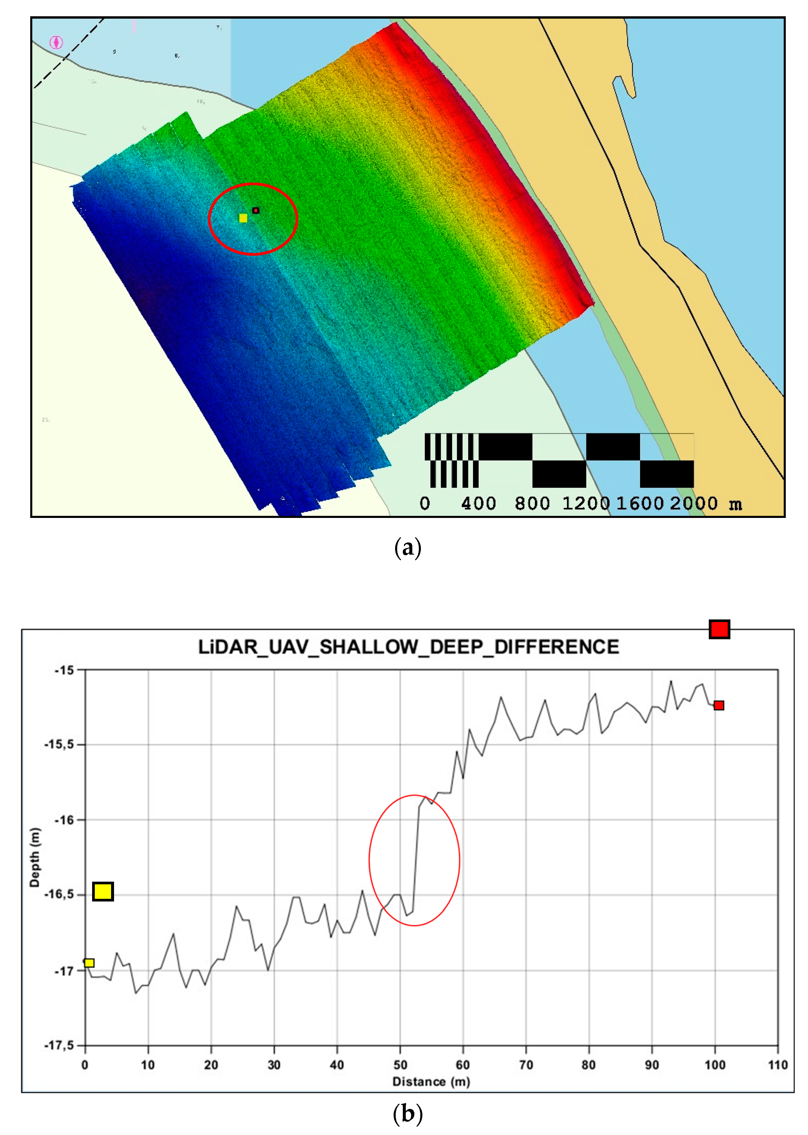
Figure 17.
SDB average in meters.
Figure 17.
SDB average in meters.
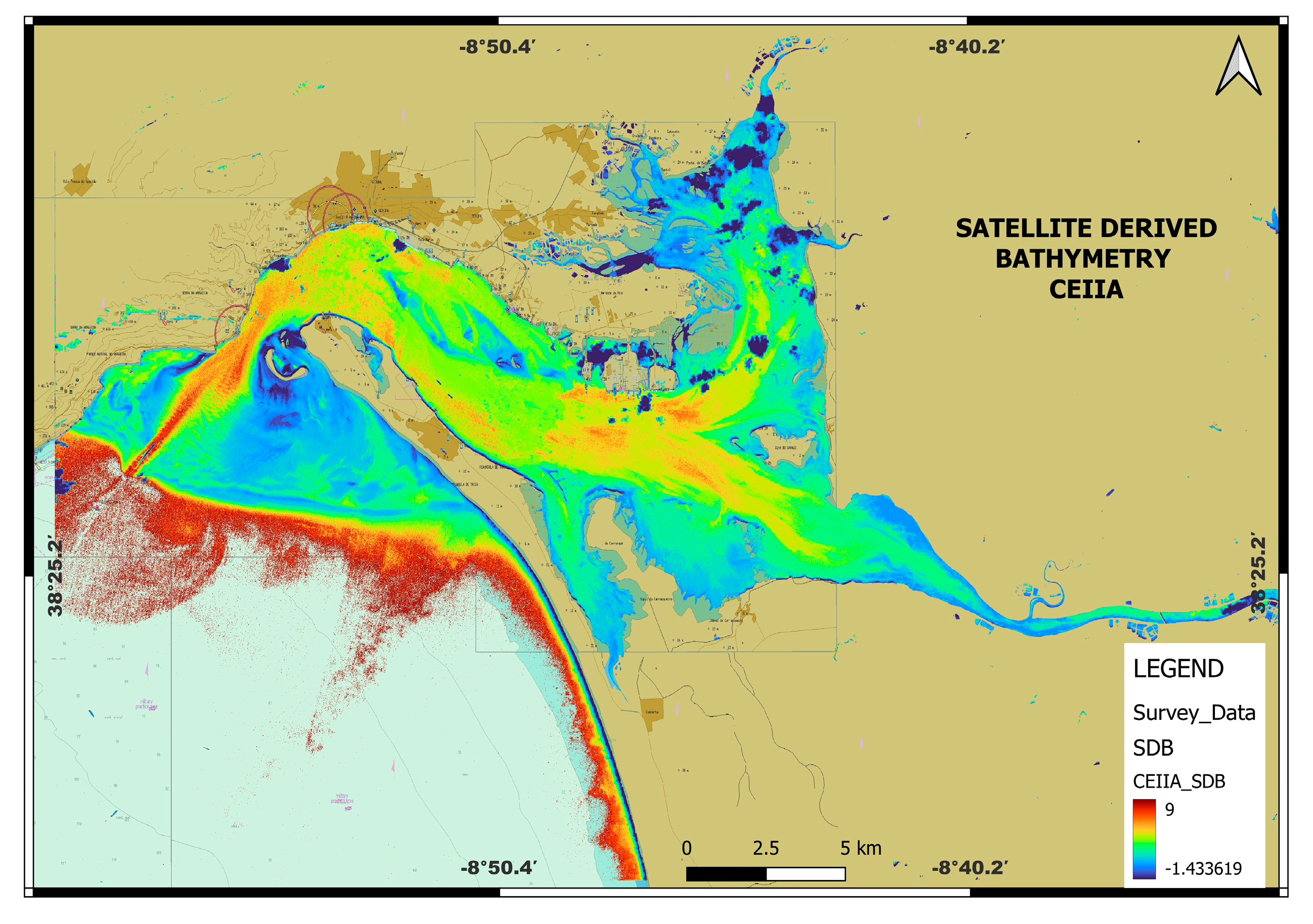
Figure 18.
Assessment of horizontal accuracy of bathymetric surfaces. (A)—MB USV, LiDAR UAV and reference survey overlay, focusing on underwater sand layers, (Second)—focuses on the same underwater sand layer, showing matches for all 3 surfaces.
Figure 18.
Assessment of horizontal accuracy of bathymetric surfaces. (A)—MB USV, LiDAR UAV and reference survey overlay, focusing on underwater sand layers, (Second)—focuses on the same underwater sand layer, showing matches for all 3 surfaces.
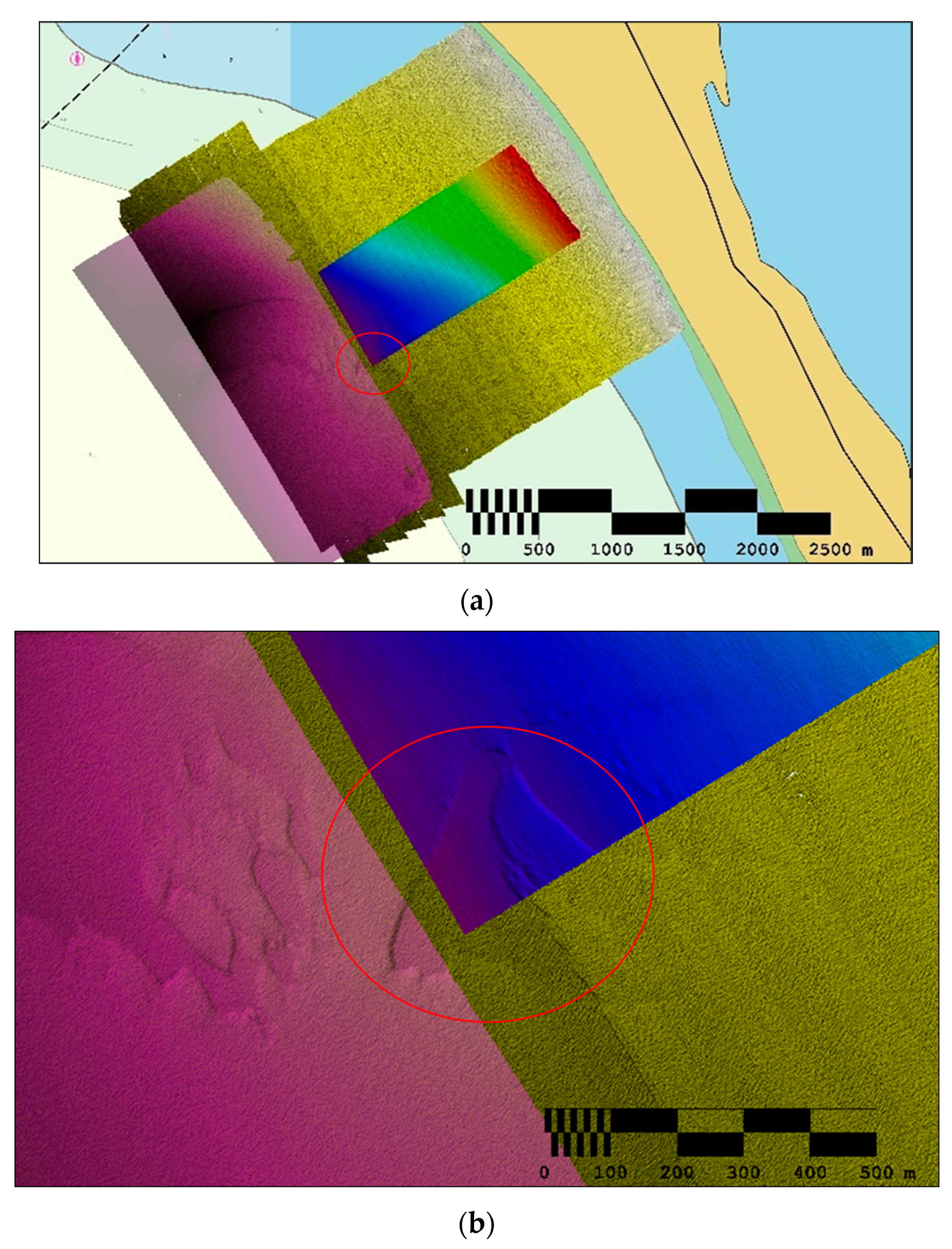
Figure 19.
Difference surface between reference measurements and drone lidar measurements.
Figure 19.
Difference surface between reference measurements and drone lidar measurements.
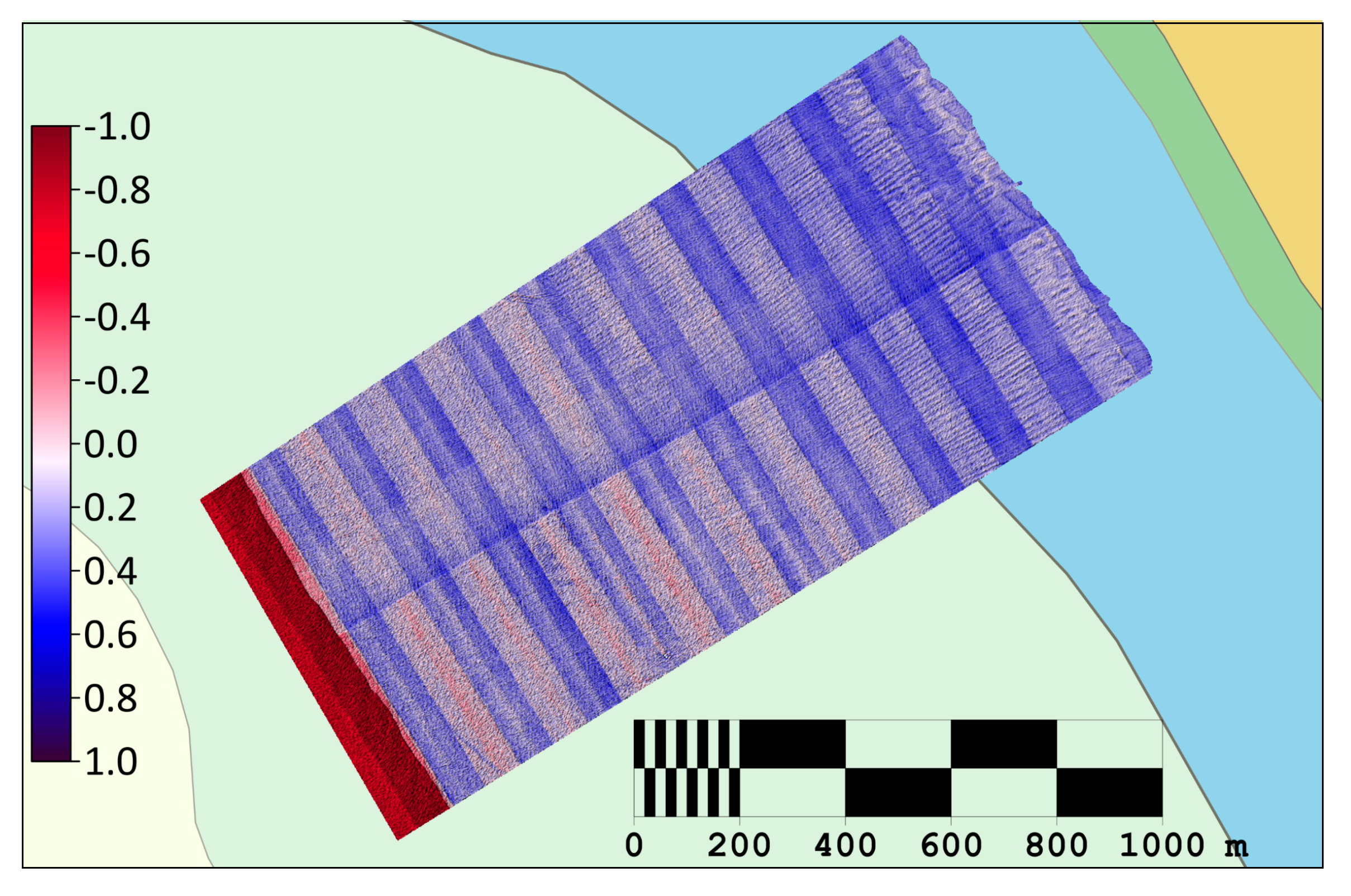
Figure 20.
LiDAR drone along-track artifacts are displayed at 20x vertical magnification.
Figure 20.
LiDAR drone along-track artifacts are displayed at 20x vertical magnification.
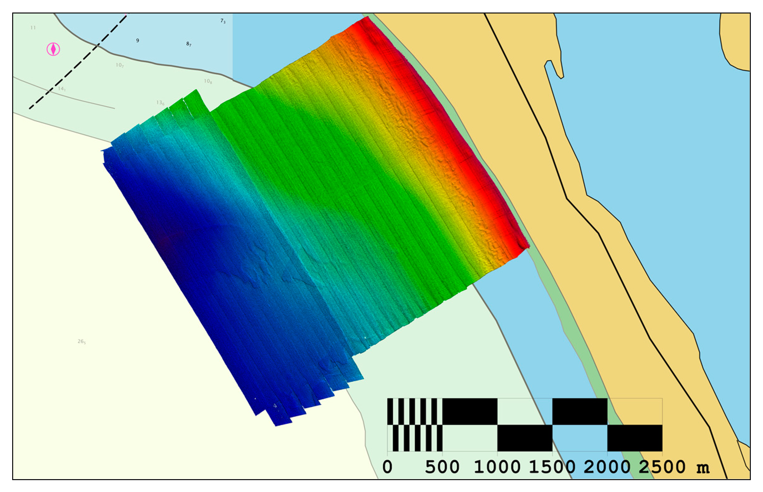
Figure 21.
Differences between reference surveys and SDB.
Figure 21.
Differences between reference surveys and SDB.
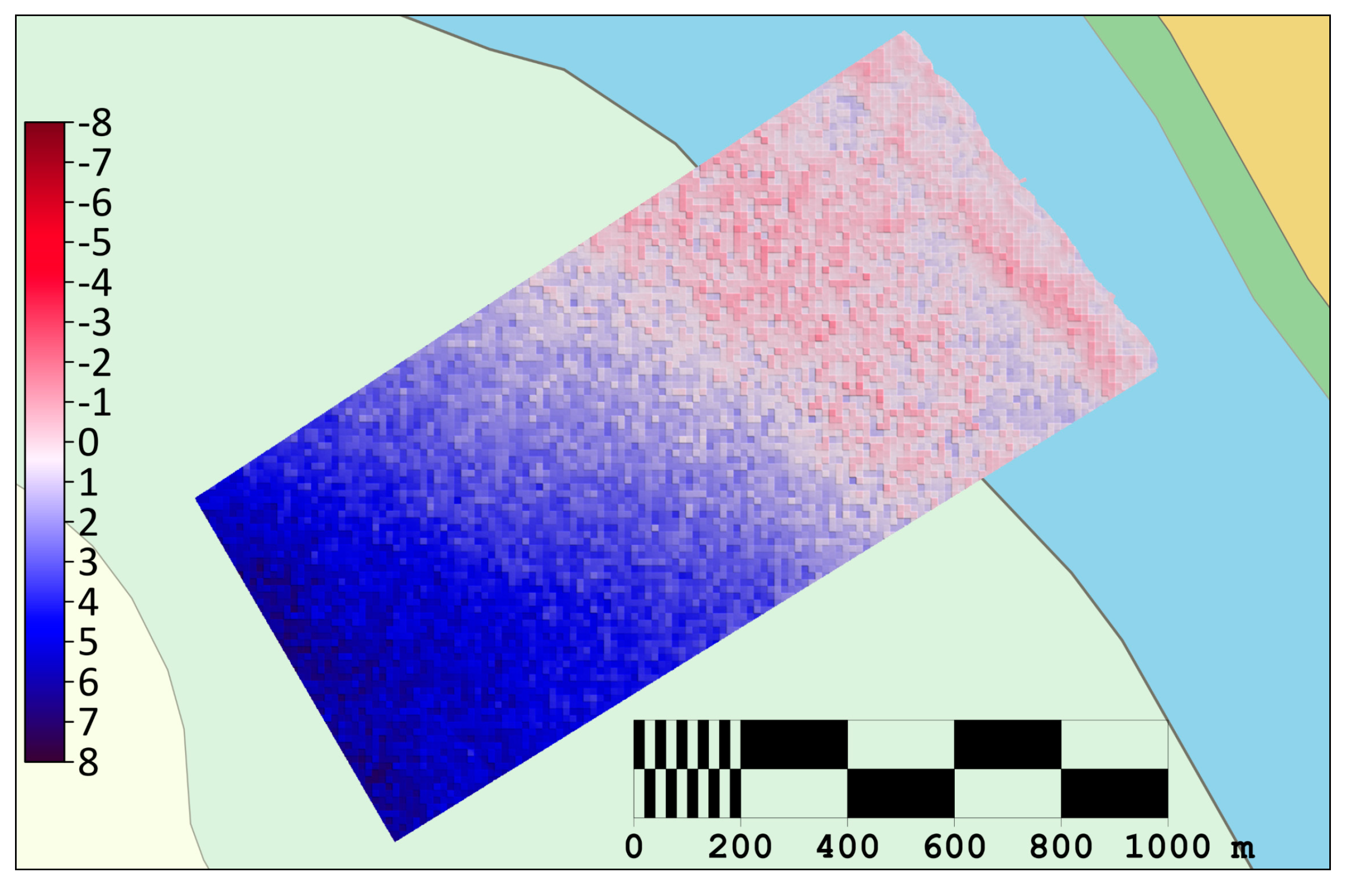
Figure 22.
Differences between UAV lidar measurements and USV MB measurements.
Figure 22.
Differences between UAV lidar measurements and USV MB measurements.
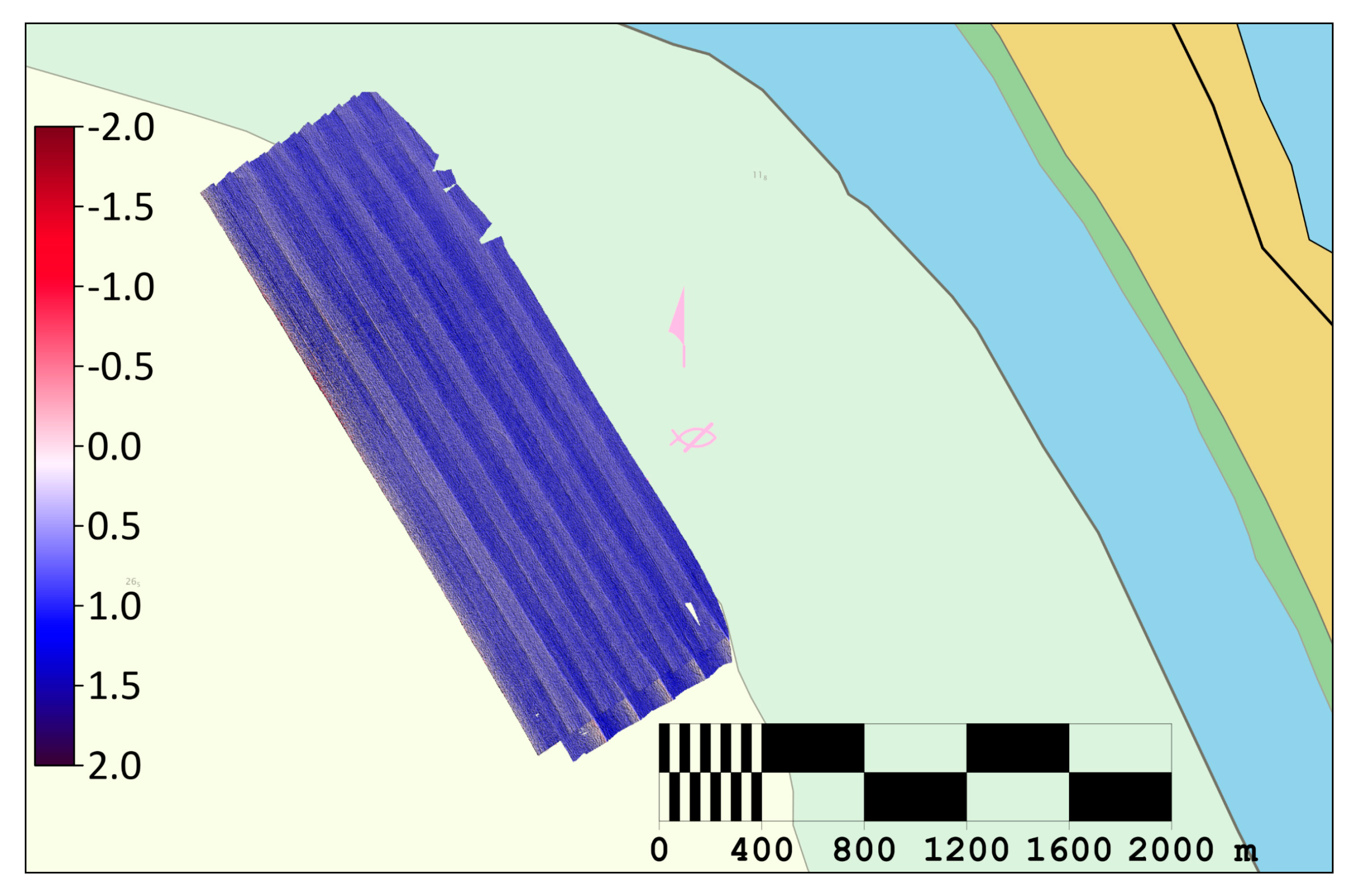
Figure 23.
LiDAR UAV and SDB surface difference versus reference measurement histograms.
Figure 23.
LiDAR UAV and SDB surface difference versus reference measurement histograms.
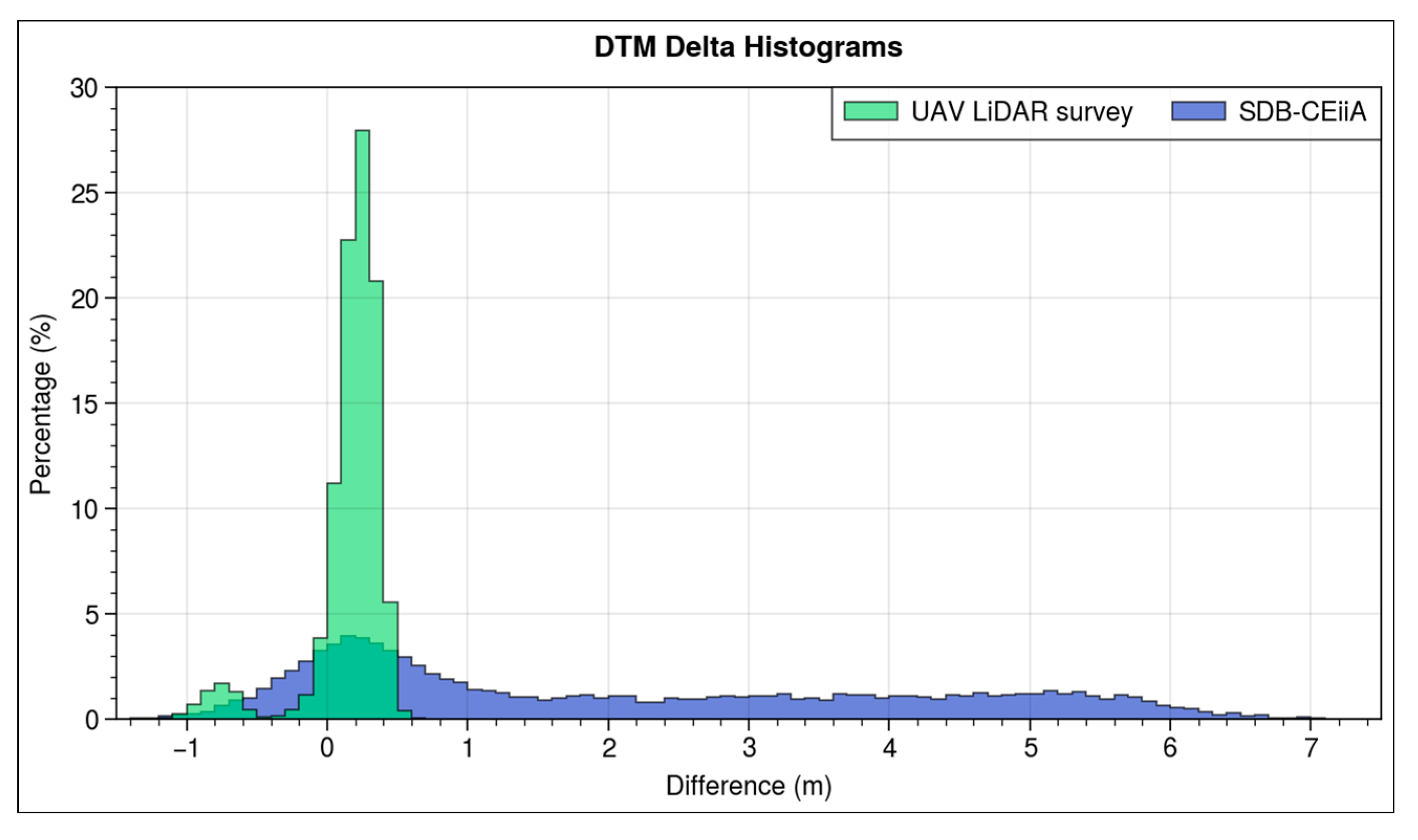
Figure 24.
Vertical profile differences between reference measurements, UAV LiDAR, USV MBES and SDB.
Figure 24.
Vertical profile differences between reference measurements, UAV LiDAR, USV MBES and SDB.
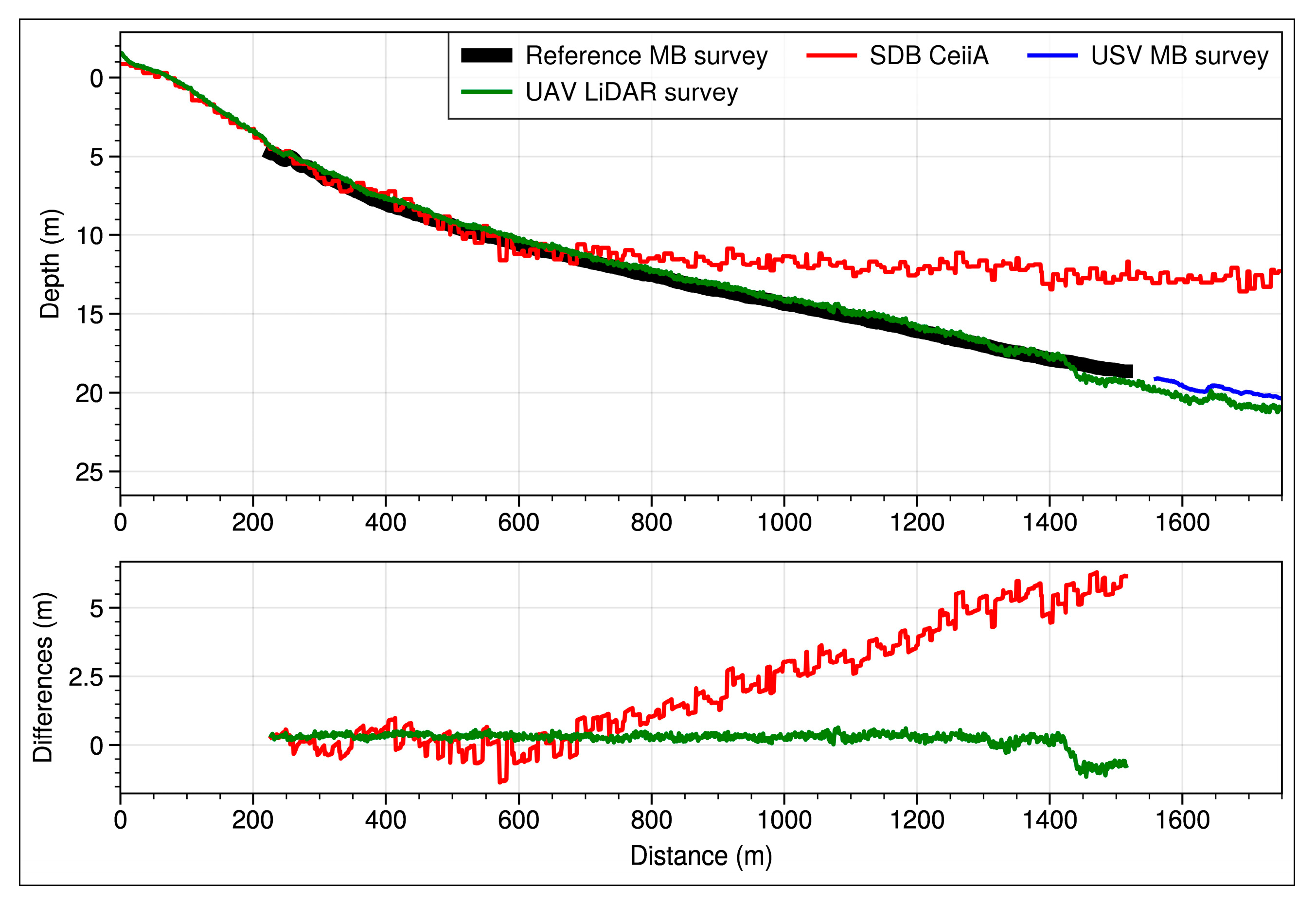
Figure 25.
Reference surface depth contours and ENC depth contours.
Figure 25.
Reference surface depth contours and ENC depth contours.
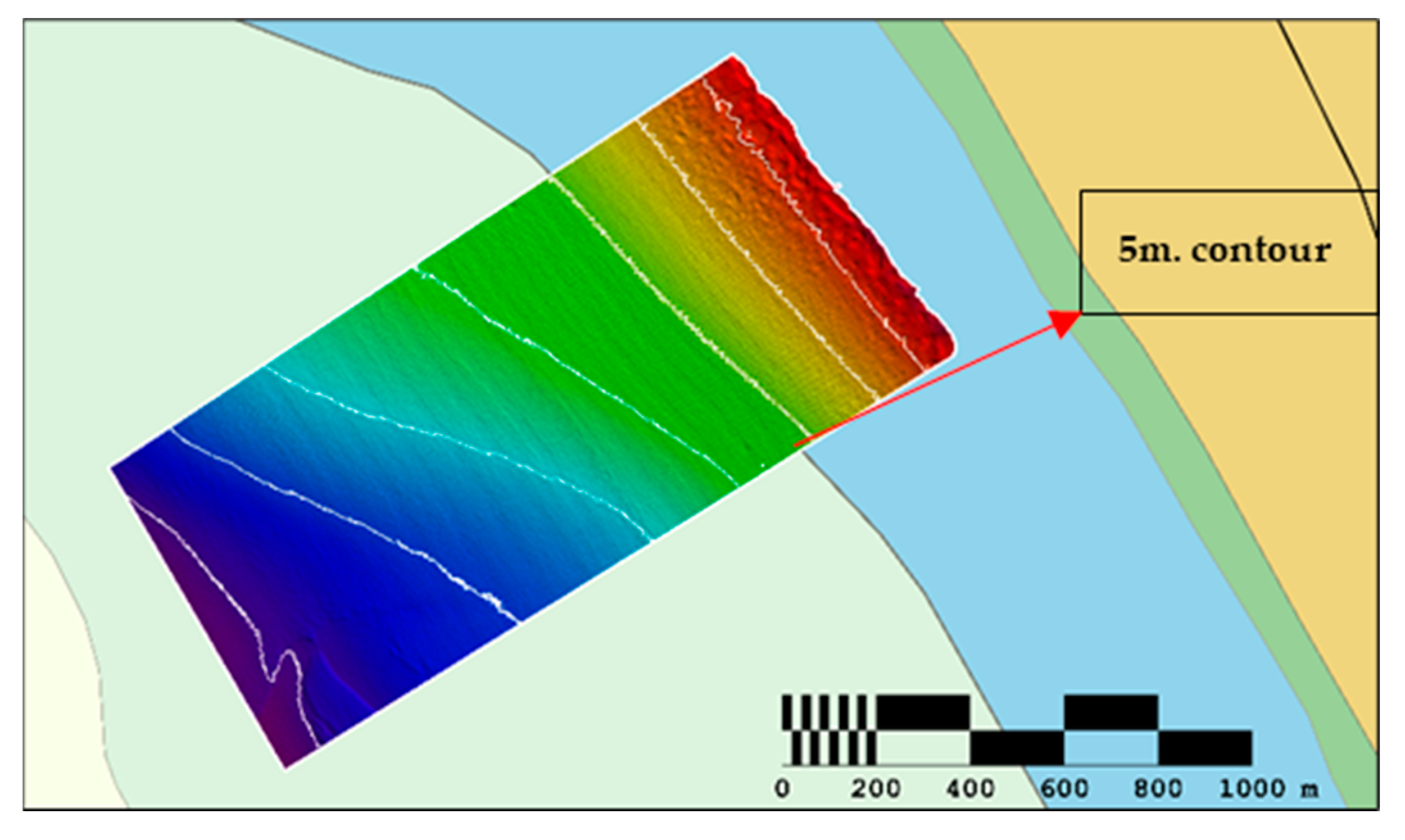
Figure 26.
MBES USV depth contours and ENC depth contours.
Figure 26.
MBES USV depth contours and ENC depth contours.
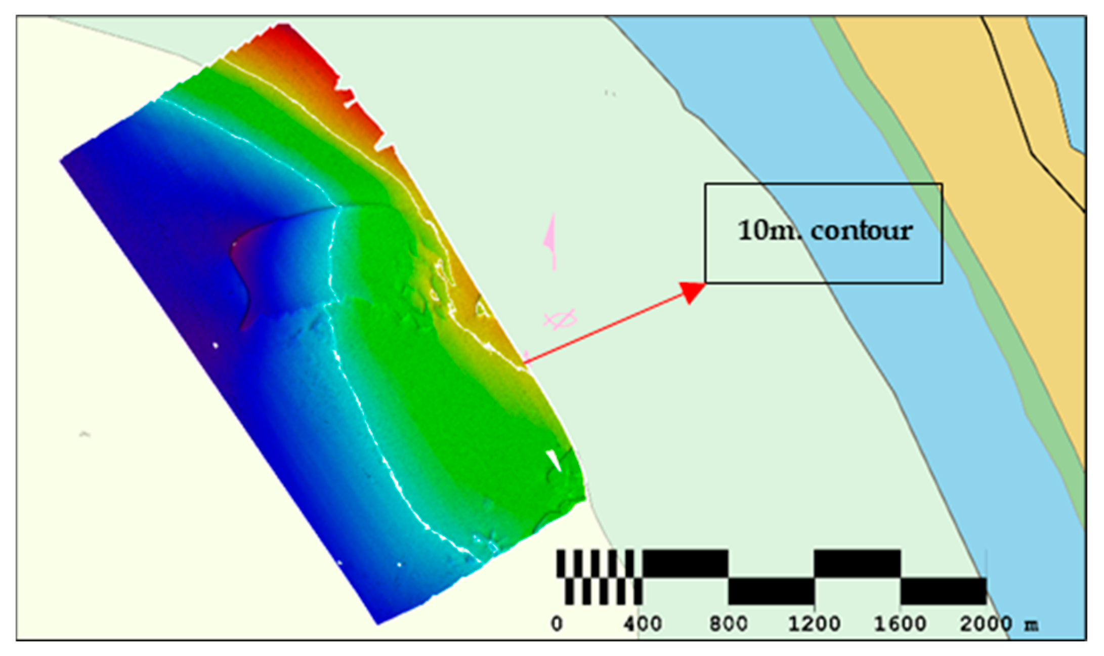
Figure 27.
LiDAR UAV depth contours and ENC depth contours.
Figure 27.
LiDAR UAV depth contours and ENC depth contours.
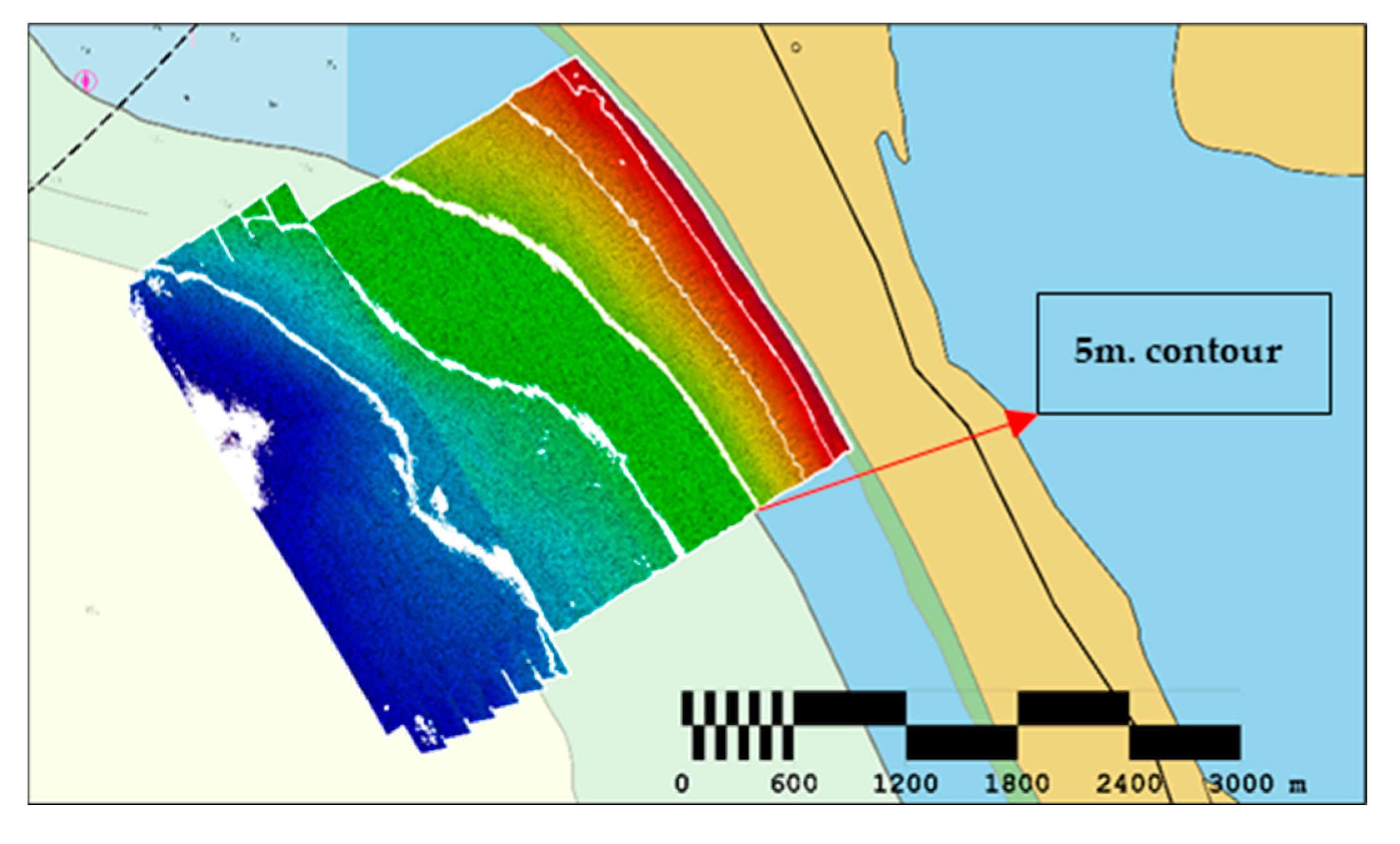
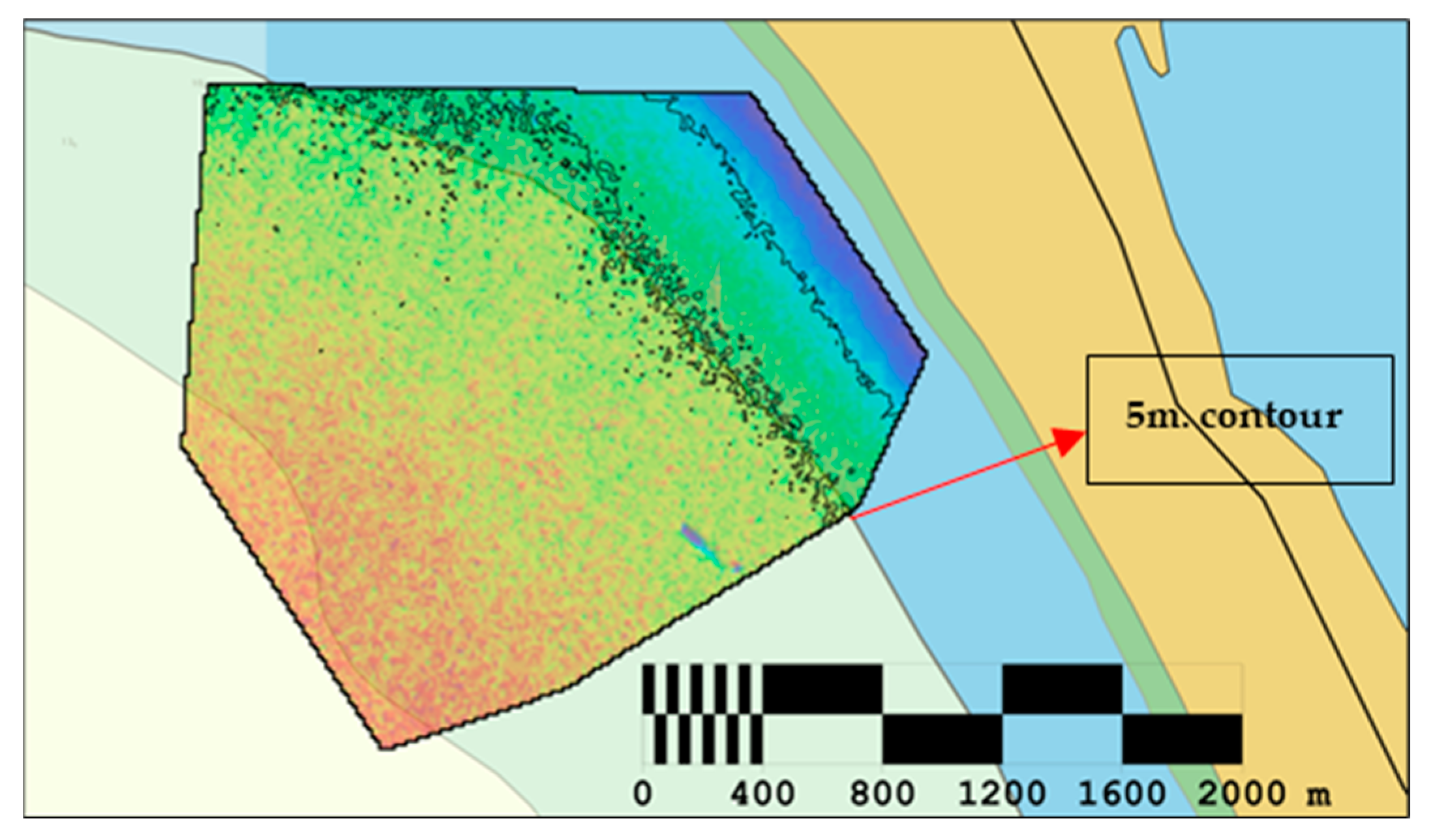
Figure 28.
SDB depth contours and ENC depth contours.
Figure 28.
SDB depth contours and ENC depth contours.
PILLS Topographic Bathymetric LiDAR Technical Specifications [39].
PILLS Topographic Bathymetric LiDAR Technical Specifications [39].
| Technical specifications | Technical specification value |
|---|---|
| aspect | 41″ x 10″ x 6″ (LxWxD) | < 2 sq. ft. volume |
| weight | <13.6 kg (30 lbs) |
| strength | <250 watts |
| Transmission specifications | Wavelength: 532 nm | Repetition rate: 30Hz×2 Energy per pulse: 37 mJ | Pulse width: 5.1 nanoseconds |
| operating height | 300 meters |
| Width | 0.9 nominal height |
| Running speed | Manned: 100–120 knots | Unmanned: 50–60 knots |
| Regional search rate | Manned: 57 km2/h | Unmanned: 31 km2/h |
| deep penetration | 3×d−1 |
| range of working temperature | −20°C to 50°C |
| point density | 25,000 points per second |
| Feature detection | 2 m cube feature |
| IHO command | 1A |
| platform | Small Opportunity Aircraft (Cessna Class and Above), Unmanned (Schiebel S-100, SeaHunter UAS), rotor |
Table 2.
LiDAR AITRAC laser measurement parameters.
Table 2.
LiDAR AITRAC laser measurement parameters.
| Laser parameters | values |
|---|---|
| scan rate | 60 Hz (2 laser combinations) |
| flight altitude | 128 meters |
| points across strips | 850 points/line |
| Scan width | 115 meters |
| spacing between points along the track | 35–50 cm |
| Cross track point spacing | 12cm |
| point density | 15–20 points/meter2 |
Kongsberg EM 712 USV Multi-Beam Technical Specifications [45].
Kongsberg EM 712 USV Multi-Beam Technical Specifications [45].
| Kongsberg EM712 USV technical specifications | |
|---|---|
| Frequency Range | 40 to 100 kHz |
| maximum ping rate | 30 Hz |
| Strip coverage | up to 140° |
| Beam spacing | Equiangular, isometric |
| roll stabilizing beam | ±15° |
| pitch stabilizer beam | ±10° |
| Sensor launch length | 970mm |
| Sensor receiving length | 970mm |
| Angular resolution | 1° × 1° (100kHz) |
| maximum. No.Number of beams per ping | 800 (dual mapping mode) |
Table 4.
Water depth measurement parameters.
Table 4.
Water depth measurement parameters.
| Refer to MB survey | USV MB Survey | Drone lidar measurement | SDB-cEiiA | |
|---|---|---|---|---|
| Total length of survey line (km) | 34.65 | 37.90 | 74.20 | – |
| Area measurement time (hours:minutes) | 02:49 | 03:17 | 02:21 | – |
| Measured average speed (knots) | 6.62 | 6.20 | 40–60 | – |
| Strip overlap(%) | 50 | 15 | 15 | – |
| Coverage area (square kilometers2) | 0.78 | 1.94 | 4.56 | 5.08 |
| Sea coverage area (%) | 15.37 | 38.21 | 89.74 | 100 |
| Measuring line spacing (meters) | 50 | 60 | 100 | – |
| Get period (day/month/year) | June 9, 2023 | 15/09/2023 | 18/09/2023 | April 1, 2023 14/04/2023 |
table 5.
Description of the bathymetric data set of the system.
table 5.
Description of the bathymetric data set of the system.
| Refer to MB survey | USV MB Survey | Drone lidar measurement | SDB-cEiiA | Shenzhen Development Bank-Airbus | |
|---|---|---|---|---|---|
| Dataset type | point cloud | point cloud | point cloud | grating | grating |
| Dataset file format | Golden Cat Mall | Golden Cat Mall | CSVXYZ | Geography TIFF | Geography TIFF |
| DTM meshing method | cube | cube | basic weighted average | – | – |
| DTM resolution (meters) | 1.00 | 1.00 | 1.00 | 10.0 | 1.20 |
Table 6.
Reference survey density and standard deviation details.
Table 6.
Reference survey density and standard deviation details.
| node density | Node standard (meters) | |
|---|---|---|
| at the lowest limit | 1 | 0.0 |
| maximum | Chapter 1683 | 0.1 |
| meaning is | 139.66 | 0.0 |
| standard deviation | 59.39 | 0.0 |
Table 7.
USV MB survey density and standard deviation details.
Table 7.
USV MB survey density and standard deviation details.
| node density | Node standard (meters) | |
|---|---|---|
| at the lowest limit | 1 | 0.0 |
| maximum | 3341 | 0.1 |
| meaning is | 110.33 | 0.0 |
| standard deviation | 61.77 | 0.0 |
Table 8.
Drone lidar measurement density and standard deviation details.
Table 8.
Drone lidar measurement density and standard deviation details.
| node density | Node standard (meters) | |
|---|---|---|
| at the lowest limit | 1 | 0.0 |
| maximum | Chapter 1173 | 2.6 |
| meaning is | 65.60 | 0.2 |
| standard deviation | 17.37 | 0.1 |
Table 9.
Surface histogram statistics for LiDAR and SDB relative to the reference survey.
Table 9.
Surface histogram statistics for LiDAR and SDB relative to the reference survey.
| Drone lidar | SDB-cEiiA | |
|---|---|---|
| Minimum (meter) | −1.3 | −1.6 |
| Maximum(m) | 0.8 | 7.2 |
| Average (meters) | 0.2 | 2.1 |
| Sexually transmitted diseases (men) | 0.3 | 2.1 |