figure 1.
Schematic representation of the geometry used in this study.
figure 1.
Schematic representation of the geometry used in this study.
figure 2.
In the data augmentation stage, LR images are created using various resolutions of the HR dataset to create the training set.
figure 2.
In the data augmentation stage, LR images are created using various resolutions of the HR dataset to create the training set.
image 3.
Open channel flow images used for training and validation. (A) Fine images (ground truth) and correspondingly scaled low-resolution images; (Second) Examples of DNS and HR image sequences at different time steps (Case 1); and (C) Example of the second set of sparse grid DNS image sequences (Case 2) used for prediction in the post-processing step.
Figure 4.
The built CNN model is UpCNN. The left branch is the encoding part, where the LR image is input, with three consecutive convolutional layers, and the right branch is the decoding part, with a deconvolutional layer that outputs the reconstructed image. The remaining connections connect information from the encoder to the decoder. Arrows indicate the direction of data flow.
Figure 5.
The range of reconstructed images for each input resolution is 5 to 25. The obtained PSNR values are also shown.
Figure 5.
The range of reconstructed images for each input resolution is 5 to 25. The obtained PSNR values are also shown.
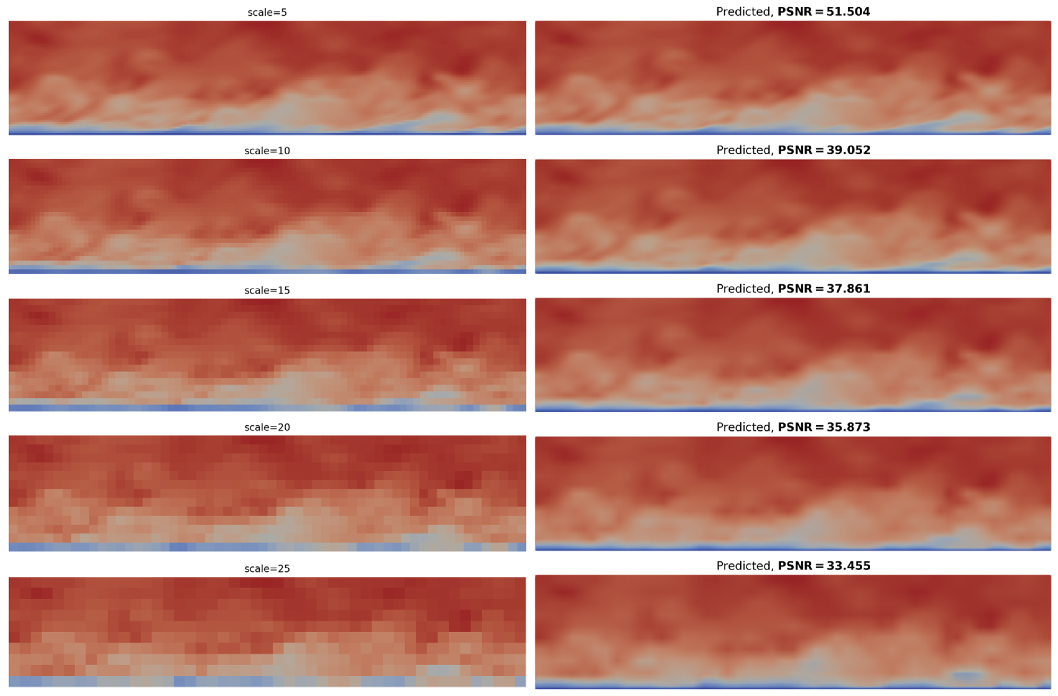
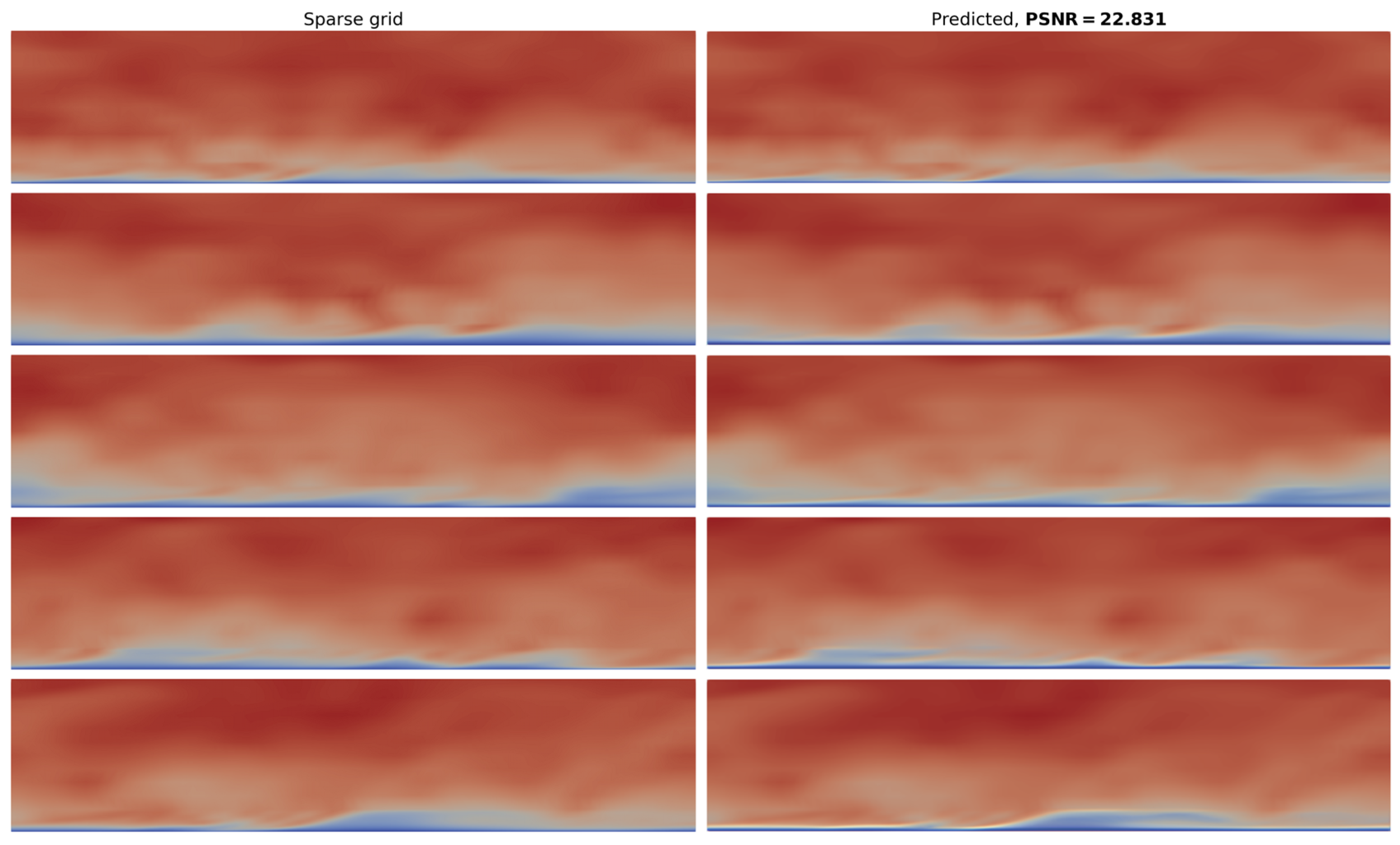
Figure 6.
Reconstructed image when sparse grid DNS input image is used as input. The obtained PSNR values (mean) are also shown.
Figure 6.
Reconstructed image when sparse grid DNS input image is used as input. The obtained PSNR values (mean) are also shown.
Enlarged version of Figure 6. The region shown is close to the fluid-solid boundary.
Enlarged version of Figure 6. The region shown is close to the fluid-solid boundary.
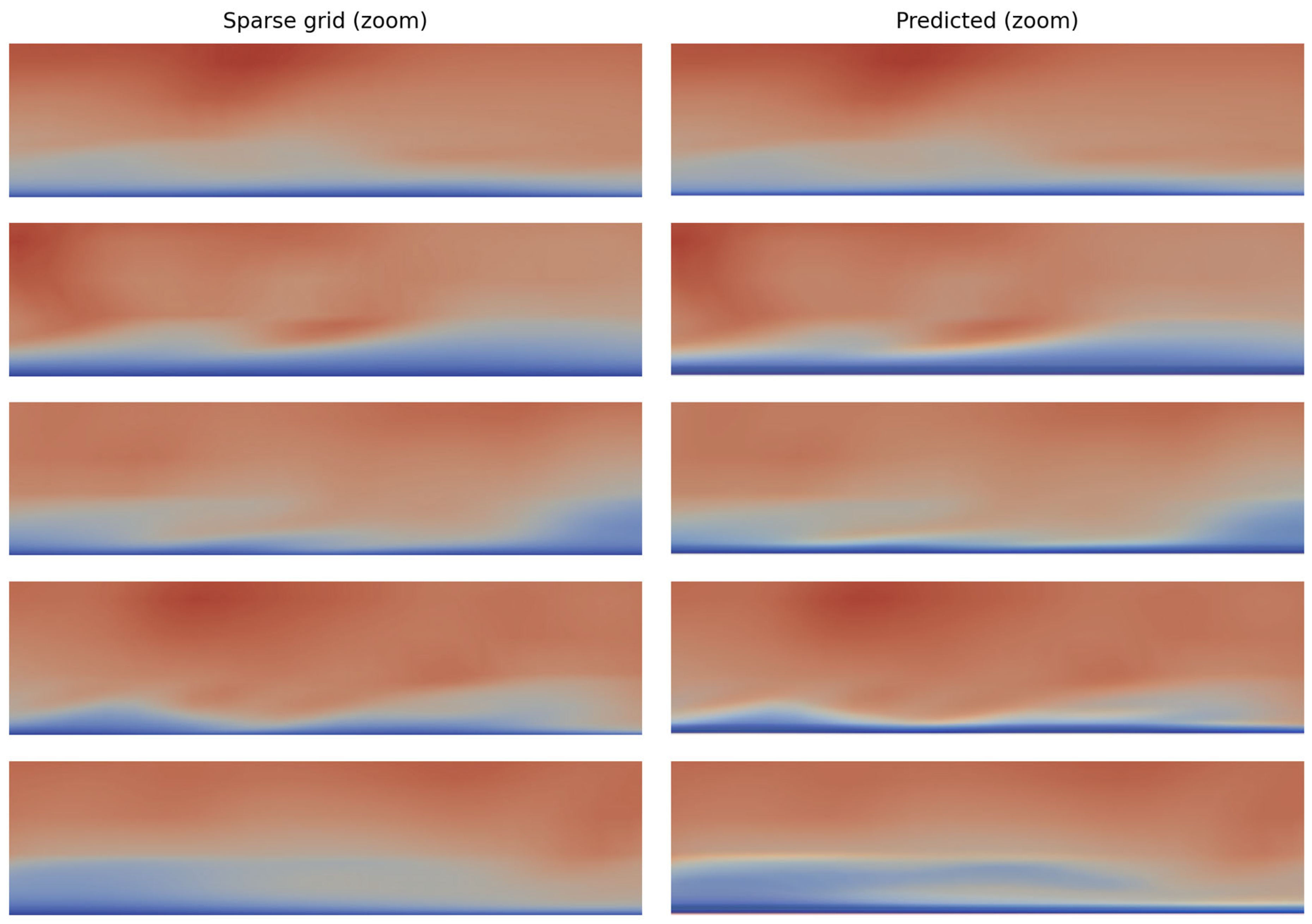
Figure 8.
(A) average flow velocity (), vertical section and (Second) identity scatter plot, where the average velocity of the HR image, compared with the average prediction speed, , for LR5. A point on the 45° line represents a perfect match.
Figure 8.
(A) average flow velocity (), vertical section and (Second) identity scatter plot, where the average velocity of the HR image, compared with the average prediction speed, , for LR5. A point on the 45° line represents a perfect match.
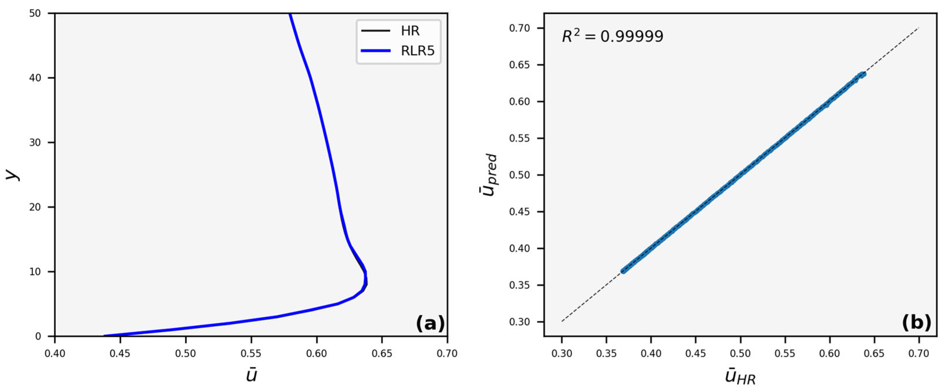
Figure 9.
(A) average flow velocity (), vertical section and (Second) identity scatter plot, where the average velocity of the HR image, compared with the average prediction speed, , for LR10. A point on the 45° line represents a perfect match.
Figure 9.
(A) average flow velocity (), vertical section and (Second) identity scatter plot, where the average velocity of the HR image, compared with the average prediction speed, , for LR10. A point on the 45° line represents a perfect match.
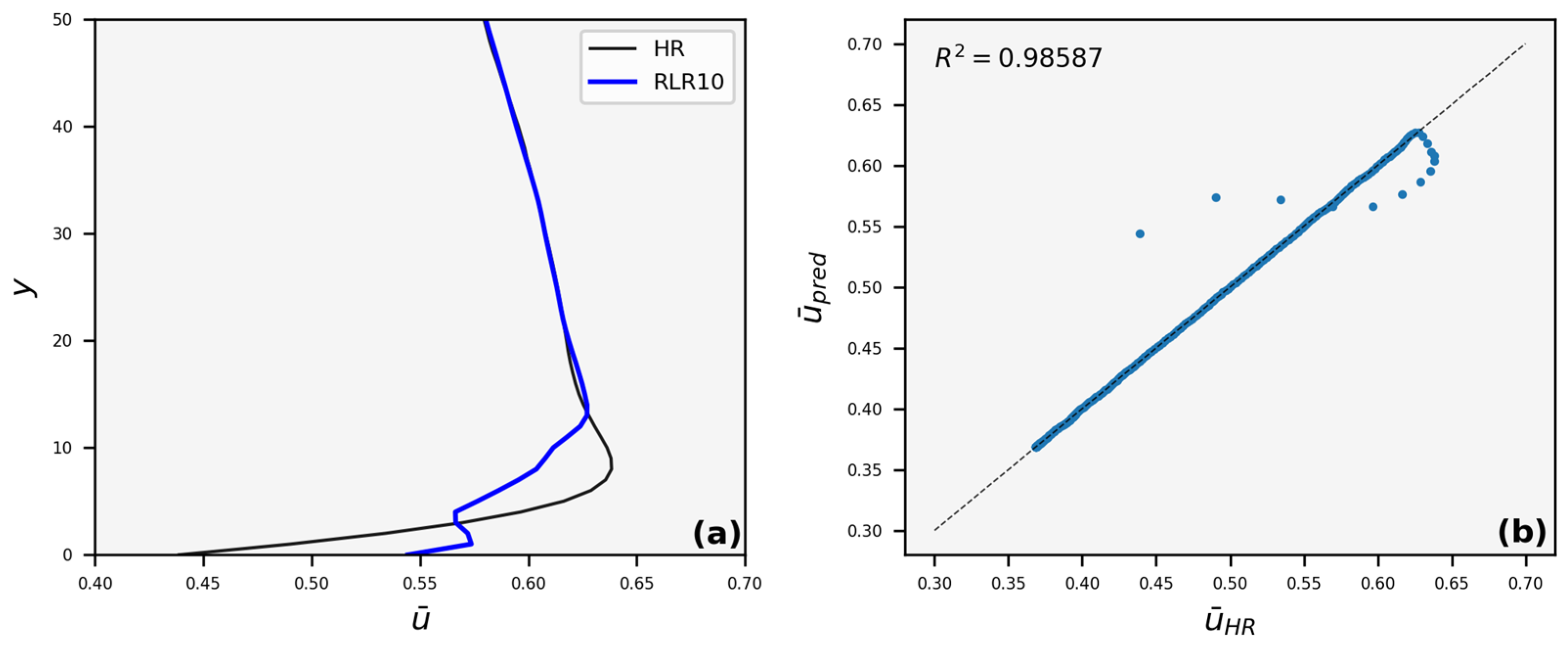
Figure 10.
(A) average flow velocity (), vertical section and (Second) identity scatter plot, where the average velocity of the HR image, compared with the average prediction speed, , for LR15. A point on the 45° line represents a perfect match.
Figure 10.
(A) average flow velocity (), vertical section and (Second) identity scatter plot, where the average velocity of the HR image, compared with the average prediction speed, , for LR15. A point on the 45° line represents a perfect match.
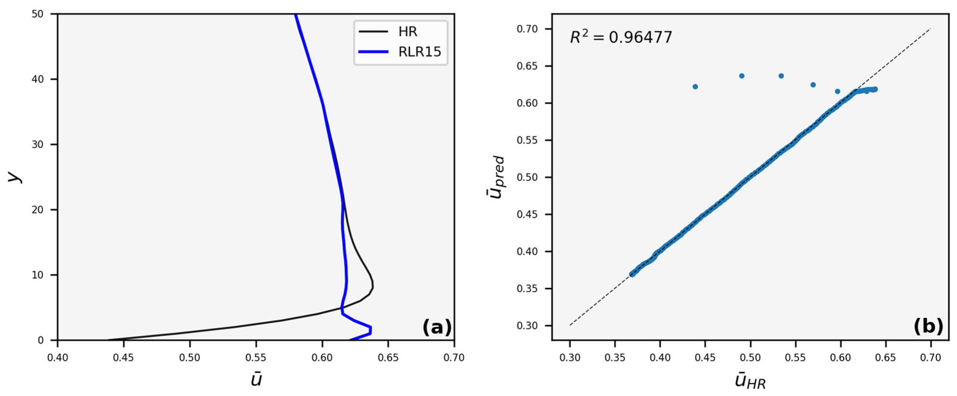
Figure 11.
(A) average flow velocity (), vertical section and (Second) identity scatter plot, where the average velocity of the HR image, compared with the average prediction speed, , for LR20. A point on the 45° line represents a perfect match.
Figure 11.
(A) average flow velocity (), vertical section and (Second) identity scatter plot, where the average velocity of the HR image, compared with the average prediction speed, , for LR20. A point on the 45° line represents a perfect match.
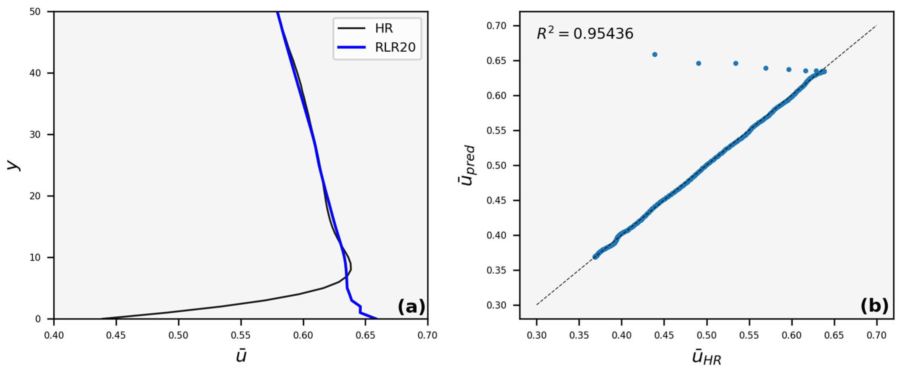
Figure 12.
(A) average flow velocity (), vertical section and (Second) identity scatter plot, where the average velocity of the HR image, compared with the average prediction speed, , for LR25. A point on the 45° line represents a perfect match.
Figure 12.
(A) average flow velocity (), vertical section and (Second) identity scatter plot, where the average velocity of the HR image, compared with the average prediction speed, , for LR25. A point on the 45° line represents a perfect match.
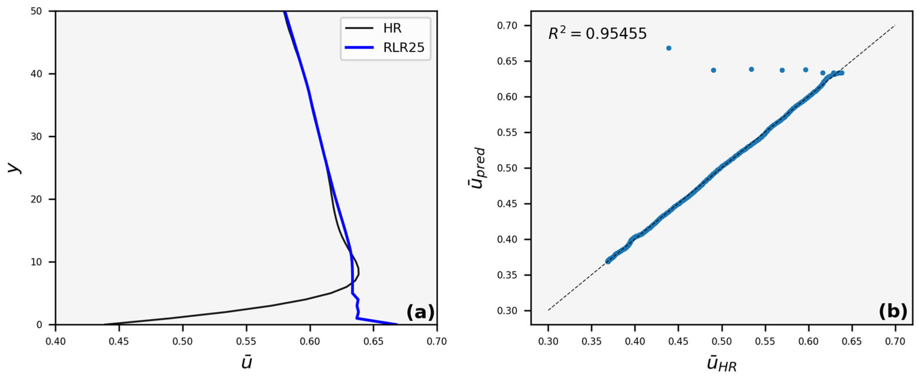
Table 1.
Input data used for model training and validation, and the number of training images (nitrogent), the number of verification images (nitrogenv) and image size (height × width). The total training set contains 200 images, and the validation set contains 50 images.
Table 1.
Input data used for model training and validation, and the number of training images (nitrogent), the number of verification images (nitrogenv) and image size (height × width). The total training set contains 200 images, and the validation set contains 50 images.
| nitrogent | nitrogenv | (Height × Width) | |
|---|---|---|---|
| human Resources | 40 | 10 | 262×1176 |
| LR5 | 40 | 10 | 52×235 |
| LR10 | 40 | 10 | 26×118 |
| LR15 | 40 | 10 | 17×78 |
| LR20 | 40 | 10 | 13×59 |
| LR25 | 40 | 10 | 10×47 |